https://habr.com/en/company/wolfram/blog/448394/- Wolfram Research corporate blog
- Cryptocurrencies
- Mathematics
- Machine learning
- Programming
Quick links
—
The Road to Version 12
—
First, Some Math
—
The Calculus of Uncertainty
—
Classic Math, Elementary and Advanced
—
More with Polygons
—
Computing with Polyhedra
—
Euclid-Style Geometry Made Computable
—
Going Super-Symbolic with Axiomatic Theories
—
The n-Body Problem
—
Language Extensions & Conveniences
—
More Machine Learning Superfunctions
—
The Latest in Neural Networks
—
Computing with Images
—
Speech Recognition & More with Audio
—
Natural Language Processing
—
Computational Chemistry
—
Geographic Computing Extended
—
Lots of Little Visualization Enhancements
—
Tightening Knowledgebase Integration
—
Integrating Big Data from External Databases
—
RDF, SPARQL and All That
—
Numerical Optimization
—
Nonlinear Finite Element Analysis
—
New, Sophisticated Compiler
—
Calling Python & Other Languages
—
More for the Wolfram “Super Shell”
—
Puppeting a Web Browser
—
Standalone Microcontrollers
—
Calling the Wolfram Language from Python & Other Places
—
Linking to the Unity Universe
—
Simulated Environments for Machine Learning
—
Blockchain (and CryptoKitty) Computation
—
And Ordinary Crypto as Well
—
Connecting to Financial Data Feeds
—
Software Engineering & Platform Updates
—
And a Lot Else…
April 16, 2019 — Stephen Wolfram
Today we’re releasing Version 12 of
Wolfram Language (and
Mathematica) on
desktop platforms, and in the
Wolfram Cloud. We released
Version 11.0 in August 2016,
11.1 in March 2017,
11.2 in September 2017 and
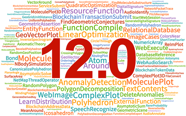
11.3 in March 2018. It’s a big jump from Version 11.3 to Version 12.0. Altogether there are
278 completely new functions, in perhaps 103 areas, together with thousands of different updates across the system:
In an “
integer release” like 12, our goal is to provide fully-filled-out new areas of functionality. But in every release we also want to deliver the latest results of our R&D efforts. In 12.0, perhaps half of our new functions can be thought of as finishing areas that were started in previous “.1” releases—while half begin new areas. I’ll discuss both types of functions in this piece, but I’ll be particularly emphasizing the specifics of what’s new in going from 11.3 to 12.0.
I must say that now that 12.0 is finished, I’m amazed at how much is in it, and how much we’ve added since 11.3. In my keynote at our
Wolfram Technology Conference last October I summarized what we had up to that point—and even that took nearly 4 hours. Now there’s even more.
What we’ve been able to do is a testament both to the strength of our R&D effort, and to the effectiveness of the Wolfram Language as a development environment. Both these things have of course been
building for three decades. But one thing that’s new with 12.0 is that we’ve been letting people watch our behind-the-scenes design process—
livestreaming more than 300 hours of my internal design meetings. So in addition to everything else, I suspect this makes Version 12.0 the very first major software release in history that’s been open in this way.
OK, so what’s new in 12.0? There are some big and surprising things—notably in
chemistry,
geometry,
numerical uncertainty and
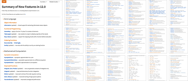
database integration. But overall, there are lots of things in lots of areas—and in fact even the basic summary of them in the
Documentation Center is already 19 pages long:
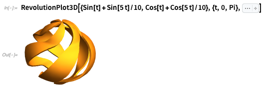
Although nowadays the vast majority of what the Wolfram Language (and Mathematica) does isn’t what’s usually considered math, we still put immense R&D effort into pushing the frontiers of what can be done in math. And as a first example of what we’ve added in 12.0, here’s the rather colorful
ComplexPlot3D:
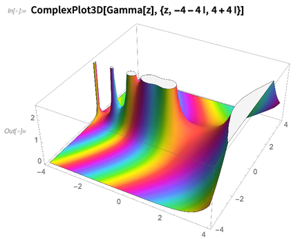
It’s always been possible to write Wolfram Language code to make plots in the complex plane. But only now have we solved the math and algorithm problems that are needed to automate the process of robustly plotting even quite pathological functions in the complex plane.
Years ago I remember
painstakingly plotting the
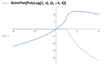
dilogarithm function, with its real and imaginary parts. Now
ReImPlot just does it:
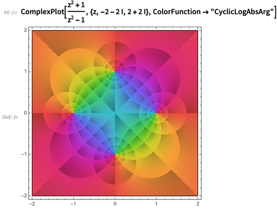
The visualization of complex functions is (pun aside) a complex story, with details making a big difference in what one notices about a function. And so one of the things we’ve done in 12.0 is to introduce carefully selected standardized ways (such as named
color functions) to highlight different features:
The Calculus of Uncertainty
Measurements in the real world often have uncertainty that gets represented as values with ± errors. We’ve had add-on packages for handling “numbers with errors” for ages. But in Version 12.0 we’re building in computation with uncertainty, and we’re doing it right.
The key is the symbolic object
Around[
x, δ], which represents a value “around
x”, with uncertainty
δ:

You can do arithmetic with
Around, and there’s a whole calculus for how the uncertainties combine:

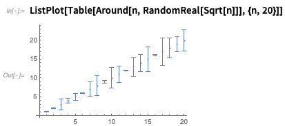
If you plot
Around numbers, they’ll be shown with error bars:
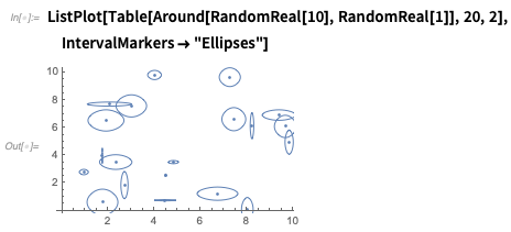
There are lots of options—like here’s one way to show uncertainty in both
x and
y:
You can have
Around quantities:

And you can also have symbolic
Around objects:

But what really is an
Around object? It’s something where there are certain rules for combining uncertainties, that are based on uncorrelated normal distributions. But there’s no statement being made that
Around[
x, δ] represents anything that actually in detail follows a normal distribution—any more than that
Around[
x, δ] represents a number specifically in the interval defined by
Interval[{
x — δ, x + δ}]. It’s just that
Around objects propagate their errors or uncertainties according to consistent general rules that successfully capture what’s typically done in experimental science.
OK, so let’s say you make a bunch of measurements of some value. You can get an estimate of the value—together with its uncertainty—using
MeanAround (and, yes, if the measurements themselves have uncertainties, these will be taken into account in weighting their contributions):

Functions all over the system—notably in
machine learning—are starting to have the option
ComputeUncertainty->
True, which makes them give
Around objects rather than pure numbers.
Around might seem like a simple concept, but it’s full of subtleties—which is the main reason it’s taken until now for it to get into the system. Many of the subtleties revolve around correlations between uncertainties. The basic idea is that the uncertainty of every
Around object is assumed to be independent. But sometimes one has values with correlated uncertainties—and so in addition to
Around, there’s also
VectorAround, which represents a vector of potentially correlated values with a specified covariance matrix.
There’s even more subtlety when one’s dealing with things like algebraic formulas. If one replaces x here with an
Around, then, following the rules of
Around, each instance is assumed to be uncorrelated:

But probably one wants to assume here that even though the value of x may be uncertain, it’s going to be same for each instance, and one can do this using the function
AroundReplace (notice the result is different):

There’s lots of subtlety in how to display uncertain numbers. Like how many trailing 0s should you put in:

Or how much precision of the uncertainty should you include (there’s a conventional breakpoint when the trailing digits are 35):

In rare cases where lots of digits are known (think, for example, some
physical constants), one wants to go to a different way to specify uncertainty:

And it goes on and on. But gradually
Around is going to start showing up all over the system. By the way, there are lots of other ways to specify
Around numbers. This is a number with 10% relative error:

This is the best
Around can do in representing an interval:

For a
distribution,
Around computes variance:

It can also take into account asymmetry by giving asymmetric uncertainties:

Classic Math, Elementary and Advanced
In making math computational, it’s always a challenge to both be able to “get everything right”, and not to confuse or intimidate elementary users. Version 12.0 introduces several things to help. First, try solving an irreducible
quintic equation:

In the past, this would have shown a bunch of explicit
Root objects. But now the
Root objects are formatted as boxes showing their approximate numerical values. Computations work exactly the same, but the display doesn’t immediately confront people with having to know about algebraic numbers.
When we say
Integrate, we mean “find an integral”, in the sense of an antiderivative. But in elementary calculus, people want to see explicit constants of integration (as they always have in
Wolfram|Alpha), so we added
an option for that (and C[
n] also has a nice, new output form):

When we benchmark our symbolic integration capabilities we do really well. But there’s always more that can be done, particularly in terms of finding the simplest forms of integrals (and at a theoretical level this is an inevitable consequence of the undecidability of symbolic expression equivalence). In Version 12.0 we’ve continued to pick away at the frontier, adding cases like:


In Version 11.3 we introduced asymptotic analysis, being able to find asymptotic values of integrals and so on. Version 12.0 adds asymptotic sums, asymptotic recurrences and asymptotic solutions to equations:


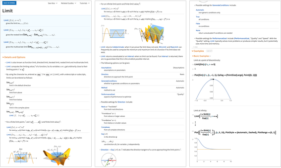
One of the great things about making math computational is that it gives us new ways to explain math itself. And something we’ve been doing is to enhance our documentation so that it explains the math as well as the functions. For example, here’s the beginning of the documentation about
Limit—with diagrams and examples of the core mathematical ideas:
Polygons have been part of the Wolfram Language since Version 1. But in Version 12.0 they’re getting generalized: now there’s a systematic way to specify holes in them. A classic geographic use case is the polygon for
South Africa—with its hole for the country of
Lesotho.
In Version 12.0, much like
Root,
Polygon gets a convenient new display form:

You can compute with it just as before:
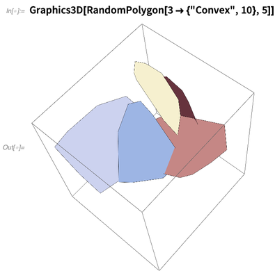
 RandomPolygon
 is new too. You can ask, say, for 5 random convex polygons, each with 10 vertices, in 3D:
There are lots of new operations on polygons. Like
PolygonDecomposition, which can, for example, decompose a polygon into convex parts:


Polygons with holes introduce a need for other kinds of operations too, like
OuterPolygon,
SimplePolygonQ, and
CanonicalizePolygon.
Polygons are pretty straightforward to specify: you just give their vertices in order (and if they have holes, you also give the vertices for the holes). Polyhedra are a bit more complicated: in addition to giving the vertices, you have to say how these vertices form faces. But in Version 12.0,
Polyhedron lets you do this in considerable generality, including voids (the 3D analog of holes), etc.
But first, recognizing their
2000+ years of history, Version 12.0 introduces functions for the five
Platonic solids:
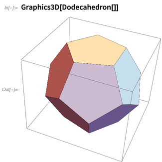
And given the Platonic solids, one can immediately start computing with them:

Here’s the solid angle subtended at vertex 1 (since it’s Platonic, all the vertices give the same angle):

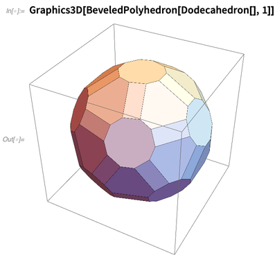
Here’s an operation done on the polyhedron:

Beyond the Platonic solids, Version 12 also builds in all the “
uniform polyhedra” (
n edges and
m faces meet at each vertex)—and you can also get symbolic
Polyhedron versions of named polyhedra from
PolyhedronData:
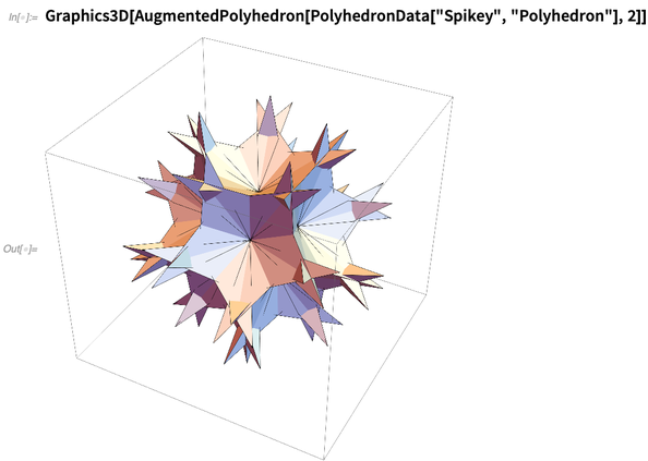
You can make any polyhedron (including a “random” one, with
RandomPolyhedron), then do whatever computations you want on it:


Mathematica and the Wolfram Language are very powerful at doing both explicit
computational geometry and
geometry represented in terms of algebra. But what about geometry the way it’s done in
Euclid’s Elements—in which one makes geometric assertions and then sees what their consequences are?
Well, in Version 12, with the whole tower of technology we’ve built, we’re finally able to deliver a new style of mathematical computation—that in effect automates what Euclid was doing 2000+ years ago. A key idea is to introduce symbolic “geometric scenes” that have symbols representing constructs such as points, and then to define geometric objects and relations in terms of them.
For example, here’s a geometric scene representing a triangle
a, b, c, and a circle through
a, b and
c, with center
o, with the constraint that
o is at the midpoint of the line from
a to
c:

On its own, this is just a symbolic thing. But we can do operations on it. For example, we can ask for a random instance of it, in which
a, b, c and
o are made specific:
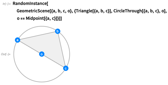
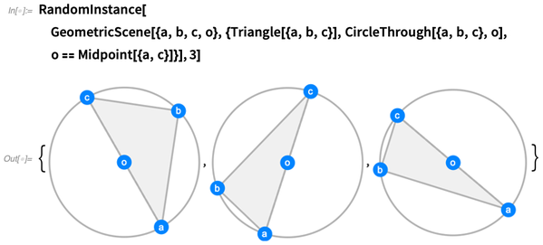
You can generate as many random instances as you want. We try to make the instances as generic as possible, with no coincidences that aren’t forced by the constraints:
OK, but now let’s “play Euclid”, and find geometric conjectures that are consistent with our setup:

For a given geometric scene, there may be many possible conjectures. We try to pick out the interesting ones. In this case we come up with two—and what’s illustrated is the first one: that the line ba is perpendicular to the line cb. As it happens, this result actually appears in Euclid (it’s in
Book 3, as part of Proposition 31)— though it’s usually called
Thales’s theorem.
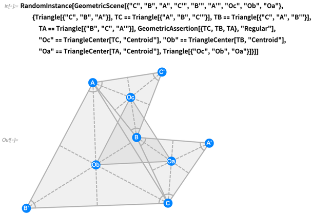
In 12.0, we now have a whole symbolic language for representing typical things that appear in Euclid-style geometry. Here’s a more complex situation—corresponding to what’s called
Napoleon’s theorem:
In 12.0 there are lots of new and useful geometric functions that work on explicit coordinates:


For triangles there are 12 types of “centers” supported, and, yes, there can be symbolic coordinates:

And to support setting up geometric statements we also need “
geometric assertions”. In 12.0 there are 29 different kinds—such as
«Parallel»,
«Congruent»,
«Tangent»,
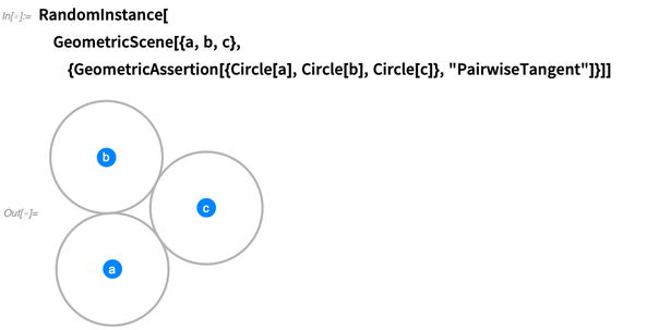
«Convex», etc. Here are three circles asserted to be pairwise tangent:
Going Super-Symbolic with Axiomatic Theories
Version 11.3 introduced
FindEquationalProof for generating symbolic representations of proofs. But what axioms should be used for these proofs? Version 12.0 introduces
AxiomaticTheory, which gives axioms for various common
axiomatic theories.
Here’s my
personal favorite axiom system:

What does this mean? In a sense it’s a more symbolic symbolic expression than we’re used to. In something like 1 +
x we don’t say what the value of
x is, but we imagine that it can have a value. In the expression above, a, b and c are pure “formal symbols” that serve an essentially structural role, and can’t ever be thought of as having concrete values.
What about the · (center dot)? In 1 +
x we know what + means. But the · is intended to be a purely abstract operator. The point of the axiom is in effect to
define a constraint on what · can represent. In this particular case, it turns out that the axiom is an
axiom for Boolean algebra, so that · can represent
Nand and
Nor. But we can derive consequences of the axiom completely formally, for example with
FindEquationalProof:

There’s quite a bit of subtlety in all of this. In the example above, it’s useful to have · as the operator, not least because it displays nicely. But there’s no built-in meaning to it, and
AxiomaticTheory lets you give something else (here
f) as the operator:

What’s the
“Nand” doing there? It’s a name for the operator (but it shouldn’t be interpreted as anything to do with the value of the operator). In the
axioms for group theory, for example, several operators appear:

This gives the default representations of the various operators here:
 AxiomaticTheory
 knows about notable theorems for particular axiomatic systems:

The basic idea of formal symbols was introduced in Version 7, for doing things like representing dummy variables in generated constructs like these:


You can enter a formal symbol using
\[FormalA] or Esc, a, Esc, etc. But back in Version 7,
\[FormalA] was rendered as
a. And that meant the expression above looked like:

I always thought this looked incredibly complicated. And for Version 12 we wanted to simplify it. We tried many possibilities, but eventually settled on single gray underdots—which I think look much better.
In
AxiomaticTheory, both the variables and the operators are “purely symbolic”. But one thing that’s definite is the arity of each operator, which one can ask
AxiomaticTheory:


Conveniently, the representation of operators and arities can immediately be fed into
Groupings, to get possible expressions involving particular variables:

The n-Body Problem
Axiomatic theories represent a classic historical area for mathematics. Another classical historical area—much more on the applied side—is the
n-body problem. Version 12.0 introduces
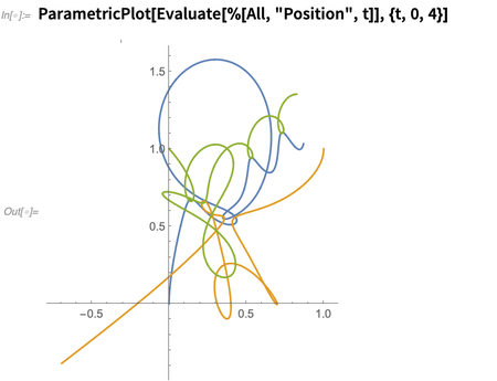
NBodySimulation, which gives simulations of the n-body problem. Here’s a three-body problem (think
Earth-Moon-Sun) with certain initial conditions (and inverse-square force law):

You can ask about various aspects of the solution; this plots the positions as a function of time:
Underneath, this is just solving differential equations, but—a bit like
SystemModel—
NBodySimulation provides a convenient way to set up the equations and handle their solutions. And, yes, standard force laws are built in, but you can define your own.
Language Extensions & Conveniences
We’ve been polishing the core of the Wolfram Language for more than 30 years now, and in each successive version we end up introducing some new extensions and conveniences.
We’ve had the function
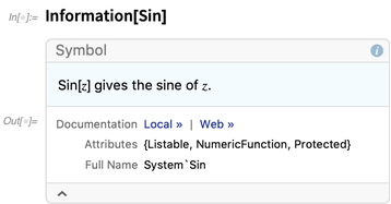
Information ever since Version 1.0, but in 12.0 we’ve greatly extended it. It used to just give information about symbols (although that’s been modernized as well):
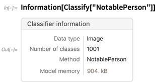
But now it also gives information about lots of kinds of objects. Here’s information on a classifier:
Here’s information about a cloud object:
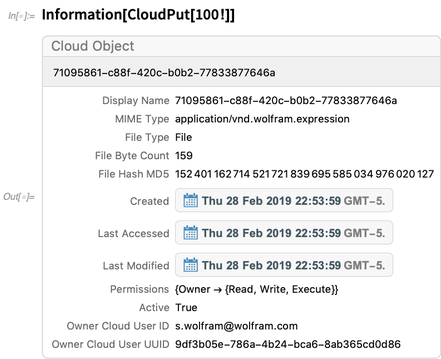
Hover over the labels in the “information box” and you can find out the names of the corresponding properties:

For entities,
Information gives a summary of known property values:
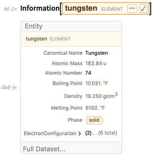
Over the past few versions, we’ve introduced a lot of new summary display forms. In Version 11.3 we introduced
Iconize, which is essentially a way of creating a summary display form for anything. Iconize has proved to be even more useful than we originally anticipated. It’s great for hiding unnecessary complexity both in notebooks and in pieces of Wolfram Language code. In 12.0 we’ve redesigned how Iconize displays, particularly to make it “read nicely” inside expressions and code.
You can explicitly iconize something:

Press the + and you’ll see some details:
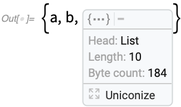
Press

and you’ll get the original expression again:

If you have lots of data you want to reference in a computation, you can always store it in a file, or in the
cloud (or even in a
data repository). It’s usually more convenient, though, to just put it in your notebook, so you have everything in the same place. One way to avoid the data “taking over your notebook” is to
put in closed cells. But Iconize provides a much more flexible and elegant way to do this.
When you’re writing code, it’s often convenient to “iconize in place”. The right-click menu now lets you do that:

Talking of display, here’s something small but convenient that we added in 12.0:

And here are a couple of other “number conveniences” that we added:


Functional programming has always been a central part of the Wolfram Language. But we’re continually looking to extend it, and to introduce new, generally useful primitives. An example in Version 12.0 is
SubsetMap:


Functions are normally things that can take several inputs, but always give a single piece of output. In areas like
quantum computing, however, one’s interested instead in having
n inputs and
n outputs.
SubsetMap effectively implements
n->n functions, picking up inputs from
n specified positions in a list, applying some operation to them, then putting back the results at the same
n positions.
I started formulating what’s now
SubsetMap about a year ago. And I quickly realized that actually I could really have used this function in all sorts of places over the years. But what should this particular “lump of computational work” be called? My initial working name was
ArrayReplaceFunction (which I shortened to
ARF in my notes). In a
sequence of (livestreamed) meetings we went back and forth. There were ideas like
ApplyAt (but it’s not really
Apply) and
MutateAt (but it’s not doing mutation in the lvalue sense), as well as
RewriteAt,
ReplaceAt,
MultipartApply and
ConstructInPlace. There were ideas about curried “function decorator” forms, like
PartAppliedFunction,
PartwiseFunction,
AppliedOnto,
AppliedAcross and
MultipartCurry.
But somehow when we explained the function we kept on coming back to talking about how it was operating on a subset of a list, and how it was really like
Map, except that it was operating on multiple elements at a time. So finally we settled on the name
SubsetMap. And—in yet another reinforcement of the importance of language design—it’s remarkable how, once one has a name for something like this, one immediately finds oneself able to reason about it, and see where it can be used.
For many years we’ve worked hard to make the Wolfram Language the highest-level and most automated system for doing
state-of-the-art machine learning. Early on, we introduced the “superfunctions”
Classify and
Predict that do
classification and prediction tasks in a completely automated way, automatically picking the best approach for the particular input given. Along the way, we’ve introduced other superfunctions—like
SequencePredict,
ActiveClassification and
FeatureExtract.
In Version 12.0 we’ve got several important new machine learning superfunctions. There’s
FindAnomalies, which finds “anomalous elements” in data:

Along with this, there’s
DeleteAnomalies, which deletes elements it considers anomalous:

There’s also
SynthesizeMissingValues, which tries to generate plausible values for missing pieces of data:

How do these functions work? They’re all based on a new function called
LearnDistribution, which tries to learn the underlying distribution of data, given a certain set of examples. If the examples were just numbers, this would essentially be a standard statistics problem, for which we could use something like
EstimatedDistribution. But the point about
LearnDistribution is that it works with data of any kind, not just numbers. Here it is learning an underlying distribution for a collection of colors:

Once we have this “learned distribution”, we can do all sorts of things with it. For example, this generates 20 random samples from it:

But now think about
FindAnomalies. What it has to do is to find out which data points are anomalous relative to what’s expected. Or, in other words, given the underlying distribution of the data, it finds what data points are outliers, in the sense that they should occur only with very low probability according to the distribution.
And just like for an ordinary numerical distribution, we can compute the
PDF for a particular piece of data. Purple is pretty likely given the distribution of colors we’ve learned from our examples:

But red is really really unlikely:

For ordinary numerical distributions, there are concepts like
CDF that tell us cumulative probabilities, say that we’ll get results that are “further out” than a particular value. For spaces of arbitrary things, there isn’t really a notion of “further out”. But we’ve come up with a function we call
RarerProbability, that tells us what the total probability is of generating an example with a smaller PDF than something we give:


Now we’ve got a way to describe anomalies: they’re just data points that have a very small rarer probability. And in fact
FindAnomalies has an option
AcceptanceThreshold (with default value 0.001) that specifies what should count as “very small”.
OK, but let’s see this work on something more complicated than colors. Let’s train an anomaly detector by looking at 1000 examples of handwritten digits:

Now
FindAnomalies can tell us which examples are anomalous:

We first introduced our symbolic framework for constructing, exploring and using neural networks back in 2016, as part of Version 11. And in every version since then we’ve added all sorts of state-of-the-art features. In June 2018 we introduced our
Neural Net Repository to make it easy to access the latest neural net models from the Wolfram Language—and already there are nearly 100 curated models of many different types in the repository, with new ones being added all the time.
So if you need the latest
BERT “transformer” neural network (that was added today!), you can get it from
NetModel:

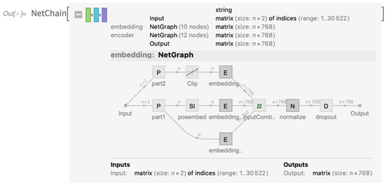
You can open this up and see the network that’s involved (and, yes, we’ve updated the display of net graphs for Version 12.0):

And you can immediately use the network, here to produce some kind of “meaning features” array:

In Version 12.0 we’ve introduced several new layer types—notably
AttentionLayer, which lets one set up the latest “transformer” architectures—and we’ve enhanced our “neural net functional programming” capabilities, with things like
NetMapThreadOperator, and multiple-sequence
NetFoldOperator. In addition to these “inside-the-net” enhancements, Version 12.0 adds all sorts of new
NetEncoder and
NetDecoder cases, such as
BPE tokenization for text in hundreds of languages, and the ability to include custom functions for getting data into and out of neural nets.
But some of the most important enhancements in Version 12.0 are more infrastructural.
NetTrain now supports
multi-GPU training, as well as dealing with mixed-precision arithmetic, and flexible early-stopping criteria. We’re continuing to use the popular
MXNet low-level neural net framework (to which we’ve been
major contributors)—so we can take advantage of the latest hardware optimizations. There are
new options for seeing what’s happening during training, and there’s also
NetMeasurements that allows you to make 33 different types of measurements on the performance of a network:

Neural nets aren’t the only—or even always the best—way to do machine learning. But one thing that’s new in Version 12.0 is that we’re now able to use
self-normalizing networks automatically in
Classify and
Predict, so they can easily
take advantage of neural nets when it makes sense.
We introduced
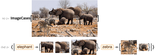
ImageIdentify, for identifying what an image is of, back in Version 10.1. In Version 12.0 we’ve managed to generalize this, to figure out not only what an image is of, but also what’s in an image. So, for example,
ImageCases will show us cases of known kinds of objects in an image:

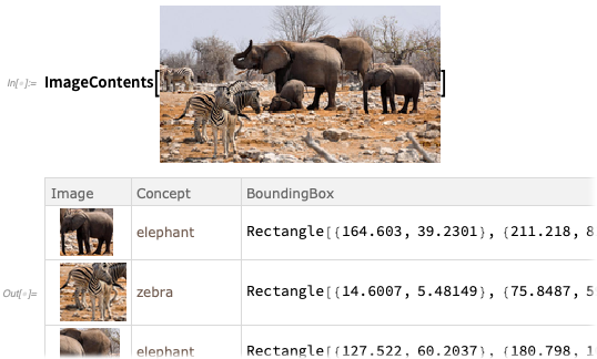
For more details,
ImageContents gives a dataset about what’s in an image:

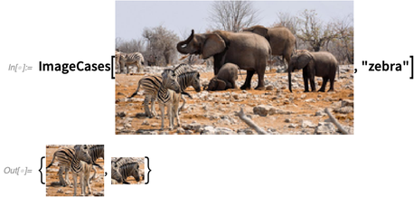
You can tell
ImageCases to look for a particular kind of thing:

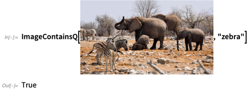
And you can also just test to see whether an image contains a particular kind of thing:

In a sense,
ImageCases is like a generalized version of
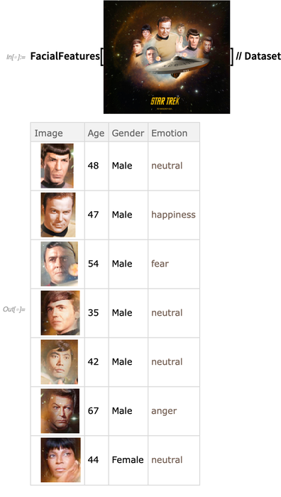
FindFaces, for finding human faces in an image. Something new in Version 12.0 is that
FindFaces and
FacialFeatures have become
more efficient and robust—with
FindFaces now based on neural networks rather than classical image processing, and the network for
FacialFeatures now being 10 MB rather than 500 MB:

Functions like
ImageCases represent “new-style” image processing, of a type that didn’t seem conceivable only a few years ago. But while such functions let one do all sorts of new things, there’s still lots of value in more classical techniques. We’ve had fairly complete
classical image processing in the Wolfram Language for a long time, but we continue to make incremental enhancements.
An example in Version 12.0 is the
ImagePyramid framework, for doing multiscale image processing:

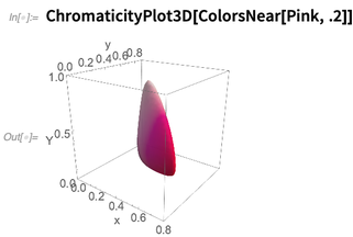
There are several new functions in Version 12.0 concerned with color computation. A key idea is
ColorsNear, which represents a neighborhood in perceptual color space, here around the color
Pink:

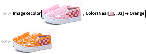
The notion of color neighborhoods can be used, for example, in the new
ImageRecolor function:

As I sit at my computer writing this, I’ll say something to my computer, and
capture it:

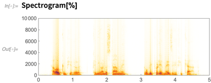
Here’s a spectrogram of the audio I captured:

So far we could do this in Version 11.3 (though
Spectrogram got 10 times faster in 12.0). But now here’s something new:

We’re doing speech-to-text! We’re using state-of-the-art neural net technology, but I’m amazed at how well it works. It’s pretty streamlined, and we’re perfectly well able to handle even very long pieces of audio, say stored in files. And on a typical computer the transcription will run at about actual real-time speed, so that an hour of speech will take about an hour to transcribe.
Right now we consider
SpeechRecognize experimental, and we’ll be continuing to enhance it. But it’s interesting to see another major computational task just become a single function in the Wolfram Language.
In Version 12.0, there are other enhancements too.
SpeechSynthesize supports new languages and new voices (as listed by
VoiceStyleData[]).
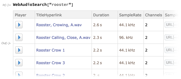
There’s now
WebAudioSearch—analogous to
WebImageSearch—that lets you search for audio on the web:

You can retrieve actual
Audio objects:

Then you can make spectrograms or other measurements:

And then—new in Version 12.0—you can use
AudioIdentify to try to identify the category of sound (is that a talking rooster?):

We still consider
AudioIdentify experimental. It’s an interesting start, but it definitely doesn’t, for example, work as well as
ImageIdentify.
A more successful audio function is
PitchRecognize, which tries to recognize the dominant frequency in an audio signal (it uses both “classical” and neural net methods). It can’t yet deal with “chords”, but it works pretty much perfectly for “single notes”.
When one deals with audio, one often wants not just to identify what’s in the audio, but to annotate it. Version 12.0 introduces the beginning of a large-scale
audio framework. Right now
AudioAnnotate can mark where there’s silence, or where there’s something loud. In the future, we’ll be adding speaker identification and word boundaries, and lots else. And to go along with these, we also have functions like
AudioAnnotationLookup, for picking out parts of an audio object that have been annotated in particular ways.
Underneath all this high-level audio functionality there’s a whole infrastructure of low-level audio processing. Version 12.0 greatly enhances
AudioBlockMap (for applying filters to audio signals), as well as introduces functions like
ShortTimeFourier.
A spectrogram can be viewed a bit like a continuous analog of a musical score, in which pitches are plotted as a function of time. In Version 12.0 there’s now
InverseSpectrogram—that goes from an array of spectrogram data to audio. Ever since Version 2 in 1991, we’ve had
Play to generate sound from a function (like
Sin[100 t]). Now with
InverseSpectrogram we have a way to go from a “frequency-time bitmap” to a sound. (And, yes, there are tricky issues about best guesses for phases when one only has magnitude information.)
Starting with
Wolfram|Alpha, we’ve had exceptionally strong
natural language understanding (NLU) capabilities for a long time. And this means that given a piece of natural language, we’re good at understanding it as Wolfram Language—that we can then go and compute from:

But what about natural language processing (NLP)—where we’re taking potentially long passages of natural language, and not trying to completely understand them, but instead just find or process particular features of them? Functions like
TextSentences,
TextStructure,
TextCases and
WordCounts have given us basic capabilities in this area for a while. But in Version 12.0—by making use of the latest machine learning, as well as our longstanding NLU and knowledgebase capabilities—we’ve now jumped to having very strong NLP capabilities.
The centerpiece is the dramatically enhanced version of
TextCases. The basic goal of
TextCases is to find cases of different types of content in a piece of text. An example of this is the classic NLP task of “entity recognition”—with
TextCases here finding what country names appear in the
Wikipedia article about ocelots:

We could also ask what islands are mentioned, but now we won’t ask for a Wolfram Language interpretation:
 TextCases
 isn’t perfect, but it does pretty well:

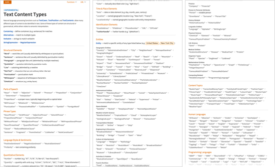
It supports a whole lot of different content types too:

You can ask it to find
pronouns, or reduced relative clauses, or
quantities, or
email addresses, or occurrences of any of 150 kinds of entities (like
companies or
plants or
movies). You can also ask it to pick out pieces of text that are in particular
human or
computer languages, or that are
about particular topics (like
travel or
health), or that have
positive or negative sentiment. And you can use constructs like
Containing to ask for combinations of these things (like noun phrases that contain the name of a river):
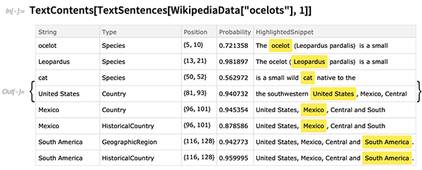
 TextContents
 lets you see, for example, details of all the entities that were detected in a particular piece of text:

And, yes, one can in principle use these capabilities through
FindTextualAnswer to try to answer questions from text—but in a case like this, the results can be pretty wacky:

Of course, you can get a real answer from our actual built-in curated knowledgebase:

By the way, in Version 12.0 we’ve added a variety of little “natural language convenience functions”, like
Synonyms and
Antonyms:

One of the “surprise” new areas in Version 12.0 is computational chemistry. We’ve had data on
explicit known chemicals in our knowledgebase for a long time. But in Version 12.0 we can compute with molecules that are specified simply as pure symbolic objects. Here’s how we can specify what turns out to be a water molecule:

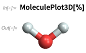
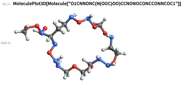
And here’s how we can make a 3D rendering:

We can deal with “known chemicals”:

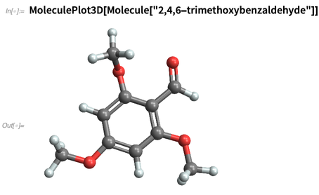
We can use arbitrary
IUPAC names:

Or we “make up” chemicals, for example specifying them by their
SMILES strings:

But we’re not just generating pictures here. We can also compute things from the structure—like symmetries:

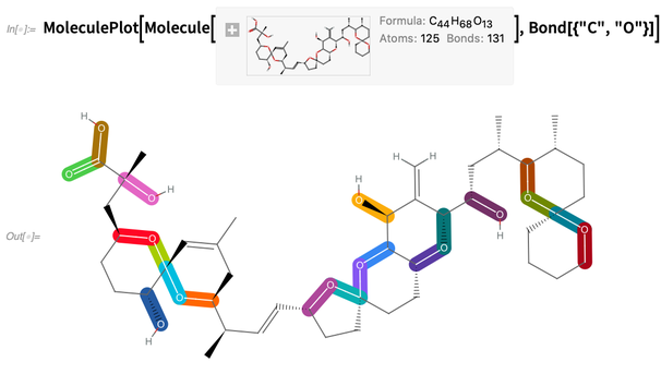
Given a molecule, we can do things like highlight carbon-oxygen bonds:

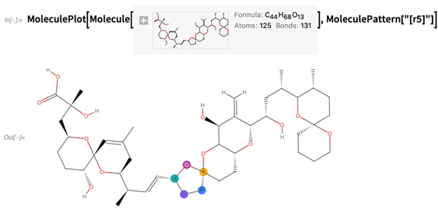
Or highlight structures, say specified by
SMARTS strings (here any 5-member ring):

You can also do searches for “molecule patterns”; the results come out in terms of atom numbers:

The computational chemistry capabilities we’ve added in Version 12.0 are pretty general and pretty powerful (with the caveat that so far they only deal with organic molecules). At the lowest level they view molecules as labeled graphs with edges corresponding to bonds. But they also know about physics, and correctly account for atomic valences and bond configurations. Needless to say, there are lots of details (about stereochemistry, symmetry, aromaticity, isotopes, etc). But the end result is that molecular structure and molecular computation have now successfully been added to the list of areas that are integrated into the Wolfram Language.
The Wolfram Language already has strong capabilities for geographic computing, but Version 12.0 adds more functions, and enhances some of those that were already there.
For example, there’s now
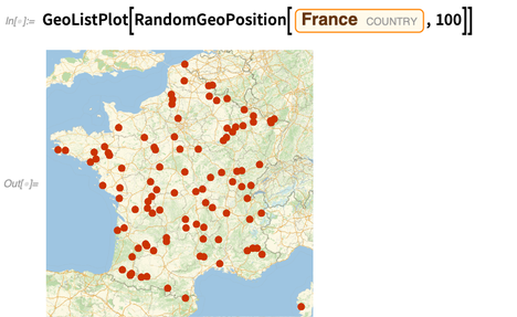
RandomGeoPosition, which generates a random lat-long location. One might think this would be trivial, but of course one has to worry about coordinate transformations—and what makes it much more nontrivial is that one can tell it to pick points only inside a certain region, here the country of France:

A theme of new geographic capabilities in Version 12.0 is handling not just geographic points and regions, but also geographic vectors. Here’s the current wind vector, for example, at the position of the Eiffel Tower, represented as a
GeoVector, with speed and direction (there’s also
GeoVectorENU, which gives east, north and up components, as well as
GeoGridVector and
GeoVectorXYZ):

Functions like
GeoGraphics let you visualize discrete geo vectors.
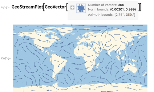
GeoStreamPlot is the geo analog of
StreamPlot (or
ListStreamPlot)—and shows streamlines formed from geo vectors (here from
WindDirectionData):

Geodesy is a mathematically sophisticated area, and we pride ourselves on doing it well in the Wolfram Language. In Version 12.0, we’ve added a few new functions to fill in some details. For example, we now have functions like
GeoGridUnitDistance and
GeoGridUnitArea which give the distortion (basically, eigenvalues of the Jacobian) associated with different geo projections at every position on Earth (or Moon, Mars, etc.).
One direction of visualization that we’ve been steadily developing is what one might call “meta-graphics”: the labeling and annotation of graphical things. We introduced
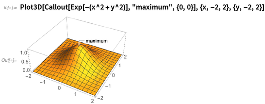
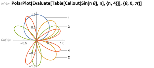
Callout in Version 11.0; in Version 12.0 it’s been extended to things like 3D graphics:

It’s pretty good at figuring out where to label things, even when they get a bit complex:

There are lots of details that matter in making graphics really look good. Something that’s been enhanced in Version 12.0 is ensuring that columns of graphics line up on their frames, regardless of the length of their tick labels. We’ve also added
LabelVisibility, which allows you to specify the relative priorities with which different labels should be made visible.
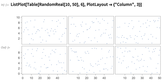
Another new feature of Version 12.0 is multipanel plot layout, where different datasets are shown in different panels, but the panels share axes whenever they can:

Tightening Knowledgebase Integration
Our curated knowledgebase—that for example powers
Wolfram|Alpha—is vast and continually growing. And with every version of the Wolfram Language we’re progressively tightening its integration into the core of the language.
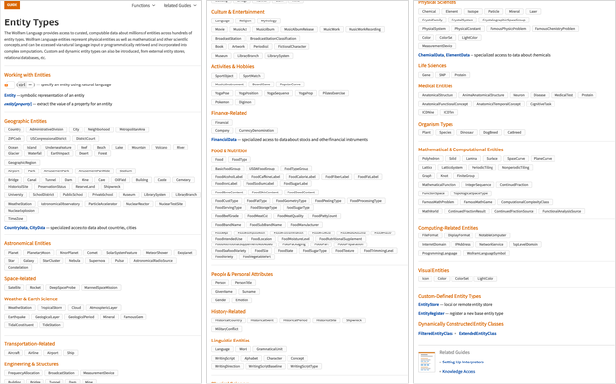
In Version 12.0 one thing we’re doing is to expose hundreds of types of entities directly in the language:

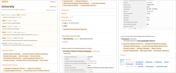
Before Version 12.0, the
Wolfram|Alpha Example pages served as a proxy for documenting many types of entities. But now there’s Wolfram Language documentation for all of them:

There are still functions like
SatelliteData,
WeatherData and
FinancialData that handle entity types that routinely need complex selection or computation. But in Version 12.0, every entity type can be accessed in the same way, with
natural language (“control + =”) input, and “yellow-boxed” entities and properties:

By the way, one can also use entities implicitly, like here asking for the 5 elements with the highest known melting points:

And one can use
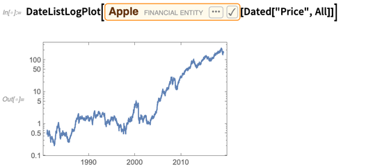
Dated to get a time series of values:

We’ve made it really convenient to work with data that’s built into the
Wolfram Knowledgebase. You have entities, and it’s very easy to ask about properties and so on:

But what if you have your own data? Can you set it up so you can use it as easily as this? A
major new feature of Version 11 was the addition of
EntityStore, in which one can
define one’s own entity types, then specify entities, properties and values.
The
Wolfram Data Repository contains a
bunch of examples of entity stores. Here’s one:

It describes a single entity type: an
«SWLibraryBook». To be able to use entities of this type just like built-in entities, we “register” the entity store:

Now we can do things like ask for 10 random entities of type
«SWLibraryBook»:

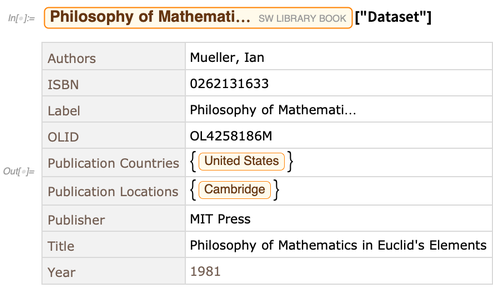
Each entity in the entity store has a variety of properties. Here’s a dataset of the values of properties for one particular entity:

OK, but with this setup we’re basically reading the whole contents of an entity store into memory. This makes it very efficient to do whatever Wolfram Language operations one wants on it. But it’s not a good scalable solution for large amounts of data—for example, data that is too big to fit in memory.
But what’s a typical source of large data? Very often it’s a database, and usually a relational one that can be accessed using
SQL. We’ve had our
DatabaseLink package for low-level read-write access to SQL databases for well over a decade. But in Version 12.0 we’re adding some major built-in features that allow external relational databases to be handled in the Wolfram Language just like entity stores, or built-in parts of the Wolfram Knowledgebase.
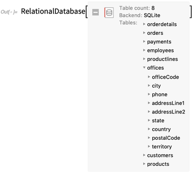
Let’s start off with a toy example. Here’s a symbolic representation of a small relational database that happens to be stored in a file:

Immediately we get a box that summarizes what’s in the database, and tells us that this database has 8 tables. If we open up the box, we can start inspecting the structure of those tables:

We can then set this relational database up as an entity store in the Wolfram Language. It looks very much the same as the library book entity store above, but now the actual data isn’t pulled into memory; instead it’s still in the external relational database, and we’re just defining a (“ORM-like”) mapping to entities in the Wolfram Language:

Now we can register this entity store, which sets up a bunch of entity types that (at least by default) are named after the names of the tables in the database:

And now we can do “entity computations” on these, just like we would on built-in entities in the Wolfram Knowledgebase. Each entity here corresponds to a row in the “employees” table in the database:

For a given entity type, we can ask what properties it has. These “properties” correspond to columns in the table in the underlying database:

Now we can ask for the value of a particular property of a particular entity:

We can also pick out entities by giving criteria; here we’re asking for “payments” entities with the 4 largest values of the “amount” property:

We can equally ask for the values of these largest amounts:

OK, but here’s where it gets more interesting: so far we’ve been looking at a little file-backed database. But we can do exactly the same thing with a giant database hosted on an external server.
As an example, let’s connect to the terabyte-sized
OpenStreetMap PostgreSQL database that contains what is basically the street map of the world:

As before, let’s register the tables in this database as entity types. Like most in-the-wild databases there are little glitches in the structure, which are worked around, but generate warnings:

But now we can ask questions about the database—like how many geo points or “nodes” there are in all the streets of the world (and, yes, it’s a big number, which is why the database is big):

Here we’re asking for the names of the objects with the 10 largest (projected) areas in the (101 GB) planet_osm_polygon table (and, yes, it takes under a second):

So how does all this work? Basically what’s happening is that our Wolfram Language representation is getting compiled into low-level SQL queries that are then sent to be executed directly on the database server.
Sometimes you’ll ask for results that are just final values (like, say, the “amounts” above). But in other cases you’ll want something intermediate—like a collection of entities that have been selected in a particular way. And of course this collection could have a billion entries. So a very important feature of what we’re introducing in Version 12.0 is that we can represent and manipulate such things purely symbolically, resolving them to something specific only at the end.
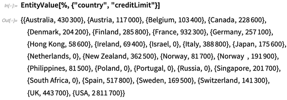
Going back to our toy database, here’s an example of how we’d specify a class of entities obtained by aggregating the total
creditLimit for all
customers with a given value of
country:

At first, this is just something symbolic. But if we ask for specific values, then actual database queries get done, and we get specific results:

There’s a family of new functions for setting up different kinds of queries. And the functions actually work not only for relational databases, but also for entity stores, and for the built-in Wolfram Knowledgebase. So, for example, we can ask for the average atomic mass for a given period in the
periodic table of elements:

An important new construct is
EntityFunction.
EntityFunction is like
Function, except that its variables represent entities (or classes of entities) and it describes operations that can be performed directly on external databases. Here’s an example with built-in data, in which we’re defining a “filtered” entity class in which the filtering criterion is a function which tests population values. The
FilteredEntityClass itself is just represented symbolically, but
EntityList actually performs the query, and resolves an explicit list of (here, unsorted) entities:


In addition to
EntityFunction,
AggregatedEntityClass and
SortedEntityClass, Version 12.0 includes
SampledEntityClass (to get a few entities from a class),
ExtendedEntityClass (to add computed properties) and
CombinedEntityClass (to combine properties from different classes). With these primitives, one can build up all the standard operations of “
relational algebra”.
In standard database programming, one typically ends up with a whole jungle of “joins” and “foreign keys” and so on. Our Wolfram Language representation lets you operate at a higher level—where basically joins become function composition and foreign keys are just different entity types. (If you want to do explicit joins, though, you can—for example using
CombinedEntityClass.)
What’s going on under the hood is that all those Wolfram Language constructs are getting compiled into SQL, or, more accurately, the specific dialect of
SQL that’s suitable for the particular database you’re using (we currently support
SQLite,
MySQL,
PostgreSQL and
MS-SQL, with support for
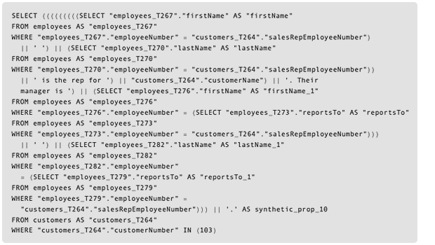
OracleSQL coming soon). When we do the compilation, we’re automatically checking types, to make sure you get a meaningful query. Even fairly simple Wolfram Language specifications can end up turning into many lines of SQL. For example,

would produce the following intermediate SQL (here for querying the SQLite database):

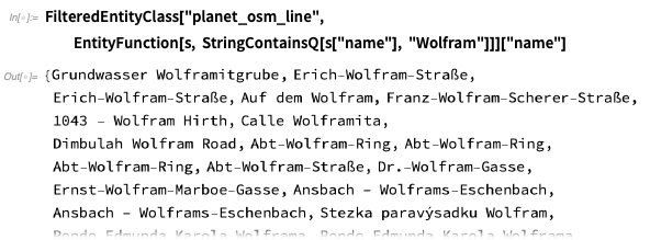
The database integration system we have in Version 12.0 is pretty sophisticated—and we’ve been working on it for quite a few years. It’s an important step forward in allowing the Wolfram Language to directly handle a new level of “bigness” in big data—and to let the Wolfram Language directly do data science on terabyte-sized datasets and beyond. Like finding which street-like entities in the world have “Wolfram” in their name:

What is the best way to represent knowledge about the world? It’s an issue that’s been debated by philosophers (and others) since antiquity. Sometimes people said logic was the key. Sometimes mathematics. Sometimes relational databases. But now we at least know one solid foundation (or at least, I’m pretty sure we do): everything can be represented by computation. This is a powerful idea—and in a sense that’s what makes everything we do with Wolfram Language possible.
But are there subsets of general computation that are useful for representing at least certain kinds of knowledge? One that we use extensively in the
Wolfram Knowledgebase is the notion of entities (“New York City”), properties (“population”) and their values (“8.6 million people”). Of course such triples don’t represent all knowledge in the world (“what will the position of Mars be tomorrow?”). But they’re a decent start when it comes to certain kinds of “static” knowledge about distinct things.
So how can one formalize this kind of knowledge representation? One answer is through graph databases. And in Version 12.0—in alignment with many
“semantic web” projects—we’re supporting
graph databases using
RDF, and queries against them using
SPARQL. In RDF the central object is an
IRI (“Internationalized Resource Identifier”), that can represent an entity or a property. A “
triplestore” then consists of a collection of triples (“subject”, “predicate”, “object”), with each element in each triple being an IRI (or a literal, such as a number). The whole object can then be thought of as a graph database or graph store, or, mathematically, a hypergraph. (It’s a
hypergraph because the predicate “edges” can also be vertices elsewhere.)
You can build your own
RDFStore much like you build an
EntityStore—and in fact you can query any Wolfram Language
EntityStore using SPARQL just like you query an
RDFStore. And since the entity-property part of the Wolfram Knowledgebase can be treated as an entity store, you can also query this. So here, finally, is an example. The country-city list
Entity["
Country"],
Entity["
City"]} in effect represents an RDF store. Then
SPARQLSelect is an operator acting on this store. What it does is to try to find a triple that matches what you’re asking for, with a particular value for the “SPARQL variable” x:


Of course, there’s also a much simpler way to do this in the Wolfram Language:

But with SPARQL you can do much more exotic things—like ask what properties relate the US to Mexico:

Or whether there is a path based on the bordering country relation from Portugal to Germany:

In principle you can just write a SPARQL query as a string (a bit like you can write an SQL string). But what we’ve done in Version 12.0 is introduce a symbolic representation of SPARQL that allows computation on the representation itself, making it easy, for example, to automatically generate complex SPARQL queries. (And it’s particularly important to do this because, on their own, practical SPARQL queries have a habit of getting extremely long and ponderous.)
OK, but are there RDF stores out in the wild? It’s been a long-running hope that a large part of the web will somehow eventually be tagged enough to “become semantic” and in effect be a giant RDF store. It’d be great if this happened, but so far it definitely hasn’t. Still, there are a few public RDF stores out there, and also some RDF stores within organizations, and with our new capabilities in Version 12.0 we’re in a unique position to do interesting things with them.
An incredibly common form of problem in industrial applications of mathematics is: “What configuration minimizes cost (or maximizes payoff) if certain constraints have to be satisfied?” More than half a century ago, the so-called
simplex algorithm was invented for solving linear versions of this kind of problem, in which both the objective function (cost, payoff) and the constraints are linear functions of the variables in the problem. By the 1980s much more efficient (“interior point”) methods had been invented—and we’ve had these for doing “
linear programming” in the Wolfram Language for a long time.
But what about nonlinear problems? Well, in the general case, one can use functions like NMinimize. And they do a state-of-the-art job. But it’s a hard problem. However, some years ago, it became clear that even among nonlinear optimization problems, there’s a class of so-called convex optimization problems that can actually be solved almost as efficiently as linear ones. (“Convex” means that both the objective and the constraints involve only convex functions—so that nothing can “wiggle” as one approaches an extremum, and there can’t be any local minima that aren’t global minima.)
In Version 12.0, we’ve now got strong implementations for all the various standard classes of convex optimization. Here’s a simple case, involving minimizing a quadratic form with a couple of linear constraints:
 NMinimize
 could already do this particular problem in Version 11.3:

But if one had more variables, the old
NMinimize would quickly bog down. In Version 12.0, however,
QuadraticOptimization will continue to work just fine, up to more than 100,000 variables with more than 100,000 constraints (so long as they’re fairly sparse).
In Version 12.0 we’ve got “raw convex optimization” functions like
SemidefiniteOptimization (that handles linear matrix inequalities) and
ConicOptimization (that handles linear vector inequalities). But functions like
NMinimize and
FindMinimum will also automatically recognize when a problem can be solved efficiently by being transformed to a convex optimization form.
How does one set up convex optimization problems? Larger ones involve constraints on whole vectors or matrices of variables. And in Version 12.0 we now have functions like
VectorGreaterEqual (input as ≥) that can immediately represent these.
Partial differential equations are hard, and we’ve been working on more and more sophisticated and general ways to handle them for 30 years. We first introduced
NDSolve (for ODEs) in
Version 2, back in 1991. We had our first (1+1-dimensional) numerical PDEs by the mid-1990s. In 2003 we introduced our powerful, modular framework for handling numerical differential equations. But in terms of PDEs we were still basically only dealing with simple, rectangular regions. To go beyond that required building our whole
computational geometry system, which we introduced in Version 10. And with this, we released
our first finite element PDE solvers. In Version 11, we then generalized to
eigen problems.
Now, in Version 12, we’re introducing another major generalization: nonlinear finite element analysis. Finite element analysis involves decomposing regions into little discrete triangles, tetrahedra, etc.—on which the original PDE can be approximated by a large number of coupled equations. When the original PDE is linear, these equations will also be linear—and that’s the typical case people consider when they talk about “finite element analysis”.
But there are many PDEs of practical importance that aren’t linear—and to tackle these one needs nonlinear finite element analysis, which is what we now have in Version 12.0.
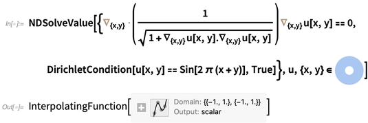
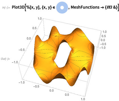
As an example, here’s what it takes to solve the nastily nonlinear PDE that describes the height of a 2D minimal surface (say, an idealized soap film), here over an annulus, with (Dirichlet) boundary conditions that make it wiggle sinusoidally at the edges (as if the soap film were suspended from wires):

On my computer it takes just a quarter of a second to solve this equation, and get an interpolating function. Here’s a plot of the interpolating function representing the solution:

We’ve put a lot of engineering into optimizing the execution of Wolfram Language programs over the years. Already in 1989 we started automatically compiling simple machine-precision numerical computations to instructions for an efficient virtual machine (and, as it happens, I wrote the original code for this). Over the years, we’ve extended the capabilities of this compiler, but it’s always been limited to fairly simple programs.
In Version 12.0 we’re taking a major step forward, and we’re releasing the first version of a new, much more powerful compiler that we’ve been working on for several years. This compiler is both able to handle a much broader range of programs (including complex functional constructs and elaborate control flows), and it’s also compiling not to a virtual machine but instead directly to optimized native machine code.
In Version 12.0 we still consider the new compiler experimental. But it’s advancing rapidly, and it’s going to have a dramatic effect on the efficiency of lots of things in the Wolfram Language. In Version 12.0, we’re just exposing a “kit form” of the new compiler, with specific compilation functions. But we’ll progressively be making the compiler operate more and more automatically—figuring out with machine learning and other methods when it’s worth taking the time to do what level of compilation.
At a technical level, the new Version 12.0 compiler is based on LLVM, and works by generating LLVM code—linking in the same low-level runtime library that the Wolfram Language kernel itself uses, and calling back to the full Wolfram Language kernel for functionality that isn’t in the runtime library.
Here’s the basic way one compiles a pure function in the current version of the new compiler:

The resulting compiled code function works just like the original function, though faster:

A big part of what lets
FunctionCompile produce a faster function is that you’re telling it to make assumptions about the type of argument it’s going to get. We’re supporting lots of basic types (like "
Integer32" and "
Real64"). But when you use
FunctionCompile, you’re committing to particular argument types, so much more streamlined code can be produced.
A lot of the sophistication of the new compiler is associated with inferring what types of data will be generated in the execution of a program. (There are lots of graph theoretic and other algorithms involved, and needless to say, all the metaprogramming for the compiler is done with the Wolfram Language.)
Here’s an example that involves a bit of type inference (the type of
fib is deduced to be
«Integer64»->«Integer64»: an integer function returning an integer):

On my computer
cf[25] runs about 300 times faster than the uncompiled function. (Of course, the compiled version fails when its output is no longer of type "
Integer64", but the standard Wolfram Language version continues to work just fine.)
Already the compiler can handle hundreds of Wolfram Language programming primitives, appropriately tracking what types are produced—and generating code that directly implements these primitives. Sometimes, however, one will want to use sophisticated functions in the Wolfram Language for which it doesn’t make sense to generate one’s own compiled code—and where what one really wants to do is just to call into the Wolfram Language kernel for these functions. In Version 12.0
KernelFunction lets one do this:

OK, but let’s say one’s got a compiled code function. What can one do with it? Well, first of all one can just run it inside the Wolfram Language. One can store it too, and run it later. Any particular compilation is done for a specific processor architecture (e.g. 64-bit x86). But
CompiledCodeFunction automatically keeps enough information to do additional compilation for a different architecture if it’s needed.
But given a
CompiledCodeFunction, one of the interesting new possibilities is that one can directly generate code that can be run even outside the Wolfram Language environment. (Our old compiler had the
CCodeGenerate package which provided slightly similar capabilities in simple cases—though even then relies on an elaborate toolchain of C compilers etc.)
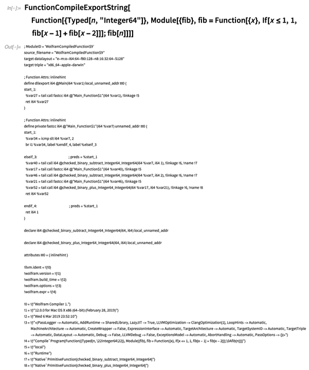
Here’s how one can export raw LLVM code (notice that things like tail recursion optimization automatically get done—and notice also the symbolic function and compiler options at the end):

If one uses
FunctionCompileExportLibrary, then one gets a library file—.dylib on Mac, .dll on Windows and .so on Linux. One can use this in the Wolfram Language by doing
LibraryFunctionLoad. But one can also use it in an external program.
One of the main things that determines the generality of the new compiler is the richness of its type system. Right now the compiler supports
14 atomic types (such as "
Boolean", "
Integer8", "
Complex64", etc.). It also supports type constructors like "
PackedArray"—so that, for example,
TypeSpecifier["
PackedArray"][
«Real64», 2] corresponds to a rank-2 packed array of 64-bit reals.
In the internal implementation of the Wolfram Language (which, by the way, is itself mostly in Wolfram Language) we’ve had an optimized way to store arrays for a long time. In Version 12.0 we’re exposing it as
NumericArray. Unlike ordinary Wolfram Language constructs, you have to tell
NumericArray in detail how it should store data. But then it works in a nice, optimized way:


In Version 11.2 we introduced
ExternalEvaluate, that lets you do computations in languages like
Python and
JavaScript from within the Wolfram Language (in
Python, “^” means
BitXor):

In Version 11.3, we introduced external language cells, to make it easy to enter external-language programs or other input directly in a notebook:

In Version 12.0, we’re tightening the integration. For example, inside an external language string, you can use <*… *> to give Wolfram Language code to evaluate:

This works in external language cells too:

Of course, Python is not Wolfram Language, so many things don’t work:

But
ExternalEvaluate can at least return many types of data from Python, including lists (as
List), dictionaries (as
Association), images (as
Image), dates (as
DateObject),
NumPy arrays (as
NumericArray) and
pandas datasets (as
TimeSeries,
DataSet, etc.). (
ExternalEvaluate can also return
ExternalObject that’s basically a handle to an object that you can send back to Python.)
You can also directly use external functions (the slightly bizarrely named ord is basically the Python analog of
ToCharacterCode):

And here’s a Python pure function, represented symbolically in the Wolfram Language:


Calling the Wolfram Language from Python & Other Places
How should one access the Wolfram Language? There are many ways. One can use it directly in a notebook. One can
call APIs that execute it in the cloud. Or one can use
WolframScript in a
command-line shell. WolframScript can run either against a local
Wolfram Engine, or against a
Wolfram Engine in the cloud. It lets you directly give code to execute:

And it lets you do things like define functions, for example with code in a file:


Along with the release of Version 12.0, we’re also releasing our first new
Wolfram Language Client Library—for Python. The basic idea of this library is to make it easy for Python programs to call the Wolfram Language. (It’s worth pointing out that we’ve effectively had a C Language Client Library for no less than 30 years—through what’s now called
WSTP.)
The way a Language Client Library works is different for different languages. For Python—as an interpreted language (that was actually historically informed by early Wolfram Language)—it’s particularly simple. After you
set up the library, and start a session (locally or in the cloud), you can then just evaluate Wolfram Language code and get the results back in Python:

You can also directly access Wolfram Language functions (as a kind of inverse of
ExternalFunction):

And you can directly interact with things like pandas structures, NumPy arrays, etc. In fact, you can in effect just treat the whole of the Wolfram Language like a giant library that can be accessed from Python. Or, of course, you can just use the nice, integrated Wolfram Language directly, perhaps creating external APIs if you need them.
More for the Wolfram “Super Shell”
One feature of using the Wolfram Language is that it lets you get away from having to think about the details of your computer system, and about things like files and processes. But sometimes one wants to work at a systems level. And for fairly simple operations, one can just use an operating system GUI. But what about for more complicated things? In the past I usually found myself using the
Unix shell. But for a long time now, I’ve instead used Wolfram Language.
It’s certainly very convenient to have everything in a notebook, and it’s been great to be able to programmatically use functions like
FileNames (ls),
FindList (grep),
SystemProcessData (ps),
RemoteRunProcess (ssh) and
FileSystemScan. But in Version 12.0 we’re adding a bunch of additional functions to support using the Wolfram Language as a “super shell”.
There’s
RemoteFile for symbolically representing a remote file (with authentication if needed)— that you can immediately use in functions like
CopyFile. There’s
FileConvert for directly converting files between different formats.
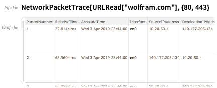
And if you really want to dive deep, here’s how you’d trace all the packets on ports 80 and 443 used in reading from
wolfram.com:

Puppeting a Web Browser
Within the Wolfram Language, it’s been easy for a long time to interact with web servers, using functions like
URLExecute and
HTTPRequest, as well as $
Cookies, etc. But in Version 12.0 we’re adding something new: the ability of the Wolfram Language to
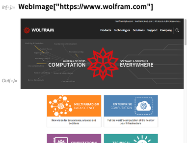
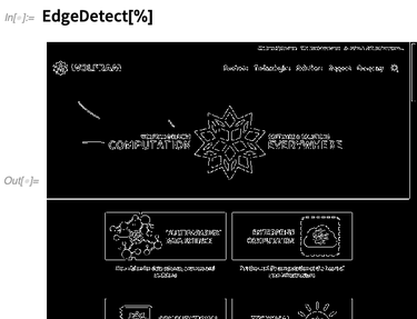
control a web browser, and programmatically make it do what we want. The most immediate thing we can do is just to get an image of what a website looks like to a web browser:

The result is an image that we can compute with:

To do something more detailed, we have to start a browser session (we currently support Firefox and Chrome):

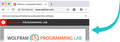
Immediately a blank browser window appears on our screen. Now we can use WebExecute to open a webpage:

Now that we’ve opened the page, there are lots of commands we can run. This clicks the first hyperlink containing the text “Programming Lab”:

This returns the title of the page we’ve reached:

You can type into fields, run JavaScript, and basically do programmatically anything you could do by hand with a web browser. Needless to say, we’ve been using a version of this technology for years inside our company to test all our various websites and web services. But now, in Version 12.0, we’re making a streamlined version generally available.
For every general-purpose computer in the world today, there are probably 10 times as many
microcontrollers—running specific computations without any general operating system. A microcontroller might cost a few cents to a few dollars, and in something like a mid-range car, there might be 30 of them.
In Version 12.0 we’re introducing a
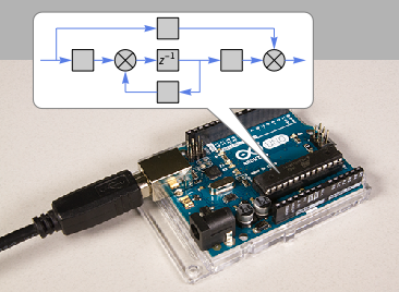
Microcontroller Kit for the Wolfram Language, that lets you give symbolic specifications from which it automatically generates and deploys code to run autonomously in microcontrollers. In the typical setup, a microcontroller is continuously doing computations on data coming in from sensors, and in real time putting out signals to actuators. The most common types of computations are effectively ones in control theory and signal processing.
We’ve had extensive support for doing
control theory and
signal processing directly in the Wolfram Language for a long time. But now what’s possible with the Microcontroller Kit is to take what’s specified in the language and download it as embedded code in a standalone microcontroller that can be
deployed anywhere (in devices, IoT, appliances, etc.).
As an example, here’s how one can generate a symbolic representation of an analog signal-processing filter:

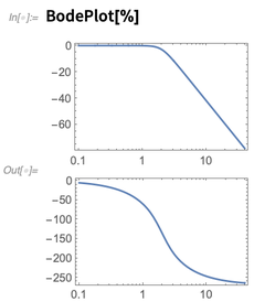
We can use this filter directly in the Wolfram Language—say using
RecurrenceFilter to apply it to an audio signal. We can also do things like plot its frequency response:

To deploy the filter in a microcontroller, we first have to derive from this continuous-time representation a discrete-time approximation that can be run in a tight loop (here, every 0.1 seconds) in the microcontroller:

Now we’re ready to use the Microcontroller Kit to actually deploy this to a microcontroller. The kit supports more than a hundred different types of microcontrollers. Here’s how we could deploy the filter to an
Arduino Uno that we have connected to a serial port on our computer:

 MicrocontrollerEmbedCode
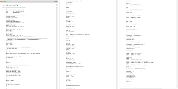
 works by generating appropriate C-like source code, compiling it for the microcontroller architecture you want, then actually deploying it to the microcontroller through its so-called programmer. Here’s the actual source code that was generated in this particular case:

So now we have a thing like this that runs our
Butterworth filter, that we can use anywhere:

If we want to check what it’s doing, we can always connect it back into the Wolfram Language using
DeviceOpen to open its
serial port, and read and write from it.
What’s the relation between the Wolfram Language and video games? Over the years, the Wolfram Language has been used behind the scenes in
many aspects of game development (simulating strategies, creating geometries, analyzing outcomes, etc.). But for some time now we’ve been working on a closer link between Wolfram Language and the
Unity game environment, and in Version 12.0 we’re releasing a first version of this link.
The basic scheme is to have Unity running alongside the Wolfram Language, then to set up two-way communication, allowing both objects and commands to be exchanged. The under-the-hood plumbing is quite complex, but the result is a nice merger of the strengths of Wolfram Language and Unity.
This sets up the link, then starts a new project in Unity:


Now create some complex shape:

Then it takes just one command to put this into the Unity game as an object called "
thingoid":

Within the Wolfram Language there’s a symbolic representation of the object, and UnityLink now provides hundreds of functions for manipulating such objects, always maintaining versions both in Unity and in the Wolfram Language.
It’s very powerful that one can take things from the Wolfram Language and immediately put them into Unity—whether they’re
geometry,
images,
audio,
geo terrain,
molecular structures,
3D anatomy, or whatever. It’s also very powerful that such things can then be manipulated within the Unity game, either through things like game physics, or by user action. (Eventually, one can expect to have
Manipulate-like functionality, in which the controls aren’t just sliders and things, but complex pieces of gameplay.)
We’ve done experiments with putting Wolfram Language–generated content into virtual reality since the early 1990s. But in modern times Unity has become something of a de facto standard for setting up VR/AR environments—and with UnityLink it’s now straightforward to routinely put things from Wolfram Language into any modern XR environment.
One can use the Wolfram Language to prepare material for Unity games, but within a Unity game UnityLink also basically lets one just insert Wolfram Language code that can be executed during a game either on a local machine or through an API in the
Wolfram Cloud. And, among other things, this makes it straightforward to put hooks into a game so the game can send “telemetry” (say to the
Wolfram Data Drop) for analysis in the Wolfram Language. (It’s also possible to script the playing of the game—which is, for example, very useful for game testing.)
Writing games is a complex matter. But UnityLink provides an interesting new approach that should make it easier to prototype all sorts of games, and to learn the ideas of game development. One reason for this is that it effectively lets one script a game at a higher level by using symbolic constructs in the Wolfram Language. But another reason is that it lets the development process be done incrementally in a notebook, and explained and documented every step of the way. For example, here’s what amounts to a
computational essay describing the development of a “
piano game”:

UnityLink isn’t a simple thing: it contains more than 600 functions. But with those functions it’s possible to access pretty much all the capabilities of Unity, and to set up pretty much any imaginable game.
For something like reinforcement learning it’s essential to have a manipulable external environment in the loop when one’s doing machine learning. Well,
ServiceExecute lets you call APIs (what’s the effect of posting that tweet, or making that trade?), and
DeviceExecute lets you actuate actual devices (turn the robot left) and get data from sensors (did the robot fall over?).
But for many purposes what one instead wants is to have a simulated external environment. And in a way, just the pure Wolfram Language already to some extent does that, for example providing access to a rich “computational universe” full of modifiable programs and equations (
cellular automata,
differential equations, …). And, yes, the things in that computational universe can be informed by the real world—say with the realistic properties of
oceans, or
chemicals or
mountains.
But what about environments that are more like the ones we modern humans typically learn in—full of built engineering structures and so on? Conveniently enough,
SystemModel gives access to lots of realistic engineering systems. And through UnityLink we can expect to have access to rich game-based simulations of the world.
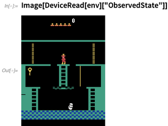
But as a first step, in Version 12.0 we’re setting up connections to some simple games—in particular from the
OpenAI “gym”. The interface is much as it would be for interacting with the real world, with the game accessed like a “device” (after appropriate sometimes-“open-source-painful” installation):

We can read the state of the game:

And we can show it as an image:

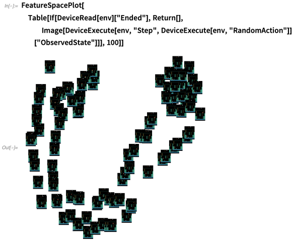
With a bit more effort, we can take 100 random actions in the game (always checking that we didn’t “die”), then show a feature space plot of the observed states of the game:

In Version 11.3 we began
our first connection to the blockchain. Version 12.0 adds a lot of new features and capabilities, perhaps most notably the ability to write to public blockchains, as well as read from them. (We also have our own
Wolfram Blockchain for Wolfram Cloud users.) We’re currently supporting
Bitcoin,
Ethereum and
ARK blockchains, both their mainnets and testnets (and, yes, we have our own nodes connecting directly to these blockchains).
In Version 11.3 we allowed
raw reading of transactions from blockchains. In Version 12.0 we’ve added a layer of analysis, so that, for example, you can ask for a summary of “CK” tokens (AKA
CryptoKitties) on the
Ethereum blockchain:

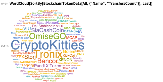
It’s quick to look at all token transactions in history, and make a word cloud of how active different tokens have been:

But what about doing our own transaction? Let’s say we want to use a
Bitcoin ATM (like the one that, bizarrely,
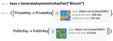
exists at a bagel store near me) to transfer cash to a Bitcoin address. Well, first we create our crypto keys (and we need to make sure we remember our private key!):

Next, we have to take our public key and generate a Bitcoin address from it:

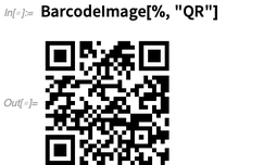
Make a QR code from that and you’re ready to go to the ATM:

But what if we want to write to the blockchain ourselves? Here we’ll use the Bitcoin testnet (so we’re not spending real money). This shows an output from a transaction we did before—that includes 0.0002 bitcoin (i.e. 20,000 satoshi):


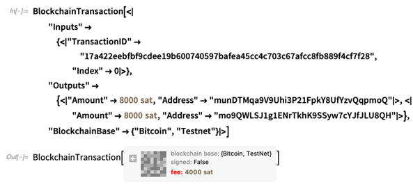
Now we can set up a transaction which takes this output, and, for example, sends 8000 satoshi to each of two addresses (that we defined just like for the ATM transaction):

OK, so now we’ve got a blockchain transaction object—that would offer a fee (shown in red because it’s “actual money” you’ll spend) of all the leftover cryptocurrency (here 4000 satoshi) to a miner willing to put the transaction in the blockchain. But before we can submit this transaction (and “spend the money”) we have to sign it with our private key:

Finally, we just apply
BlockchainTransactionSubmit and we’ve submitted our transaction to be put on the blockchain:

Here’s its transaction ID:

If we immediately ask about this transaction, we’ll get a message saying it isn’t in the blockchain:

But after we wait a few minutes, there it is—and it’ll soon spread to every copy of the Bitcoin testnet blockchain:

If you’re prepared to spend real money, you can use exactly the same functions to do a transaction on a main net. You can also do things like buy CryptoKitties. Functions like
BlockchainContractValue can be used for any (for now, only Ethereum) smart contract, and are set up to immediately understand things like
ERC-20 and
ERC-721 tokens.
Dealing with blockchains involves lots of cryptography, some of which is new in Version 12.0 (notably, handling elliptic curves). But in Version 12.0 we’re also extending our non-blockchain cryptographic functions. For example, we’ve now got functions for directly dealing with
digital signatures. This creates a digital signature using the private key from above:


Now anyone can verify the message using the corresponding public key:

In Version 12.0, we added several new types of hashes for the
Hash function, particularly to support various cryptocurrencies. We also added ways to generate and verify
derived keys. Start from any password, and
GenerateDerivedKey will “puff it out” to something longer (to be more secure you should add “
salt”):

Here’s a version of the derived key, suitable for use in various authentication schemes:

Connecting to Financial Data Feeds
The
Wolfram Knowledgebase contains all sorts of
financial data. Typically there’s a
financial entity (like a stock), then there’s a property (like price). Here’s the complete daily history of Apple’s stock price (it’s very impressive that it looks best on a log scale):

But while the financial data in the Wolfram Knowledgebase, and standardly available in the Wolfram Language, is continuously updated, it’s not real time (mostly it’s 15-minute delayed), and it doesn’t have all the detail that many financial traders use. For serious finance use, however, we’ve developed
Wolfram Finance Platform. And now, in Version 12.0, it’s got direct access to Bloomberg and Reuters financial data feeds.
The way we architect the Wolfram Language, the framework for the connections to Bloomberg and Reuters is always available in the language—but it’s only activated if you have Wolfram Finance Platform, as well as the appropriate Bloomberg or Reuters subscriptions. But assuming you have these, here’s what it looks like to connect to the
Bloomberg Terminal service:

All the financial instruments handled by the Bloomberg Terminal now become available as entities in the Wolfram Language:

Now we can ask for properties of this entity:

Altogether there are more than 60,000 properties accessible from the Bloomberg Terminal:

Here are 5 random examples (yes, they’re pretty detailed; those are Bloomberg names, not ours):

We support the Bloomberg Terminal service, the
Bloomberg Data License service, and the
Reuters Elektron service. One sophisticated thing one can now do is to set up a continuous task to asynchronously receive data, and call a “
handler function” every time a new piece of data comes in:

Software Engineering & Platform Updates
I’ve talked about lots of new functions and new functionality in the Wolfram Language. But what about the underlying infrastructure of the Wolfram Language? Well, we’ve been working hard on that too. For example, between Version 11.3 and Version 12.0 we’ve managed to fix nearly 8000 reported bugs. We’ve also made lots of things faster and more robust. And in general we’ve been tightening the software engineering of the system, for example reducing the initial download size by nearly 10% (despite all the functionality that’s been added). (We’ve also done things like improve the predictive
prefetching of knowledgebase elements from the cloud—so when you need similar data it’s more likely to be already cached on your computer.)
It’s a longstanding feature of the computing landscape that operating systems are continually getting updated—and to take advantage of their latest features, applications have to get updated too. We’ve been working for several years on a major update to our Mac notebook interface—which is finally ready in Version 12.0. As part of the update, we’ve rewritten and restructured large amounts of code that have been developed and polished over more than 20 years, but the result is that in Version 12.0, everything about our system on the Mac is fully 64-bit, and makes use of the latest
Cocoa APIs. This means that the notebook front end is significantly faster—and can also go beyond the previous 2 GB memory limit.
There’s also a platform update on Linux, where now the notebook interface fully supports
Qt 5, which allows all rendering operations to take place “headlessly”, without any X server—greatly streamlining deployment of the
Wolfram Engine in the cloud. (Version 12.0 doesn’t yet have high-dpi support for Windows, but that’s coming very soon.)
The development of the
Wolfram Cloud is in some ways separate from the development of the Wolfram Language, and
Wolfram Desktop applications (though for internal compatibility we’re releasing Version 12.0 at the same time in both environments). But in the past year since Version 11.3 was released, there’s been dramatic progress in the Wolfram Cloud.
Especially notable are the advances in cloud notebooks—supporting more interface elements (including some, like embedded websites and videos, that aren’t even yet available in desktop notebooks), as well as greatly increased robustness and speed. (Making our whole notebook interface work in a web browser is no small feat of software engineering, and in Version 12.0 there are some pretty sophisticated strategies for things like maintaining consistent fast-to-load caches, along with full symbolic DOM representations.)
In Version 12.0 there’s now just a simple menu item (File > Publish to Cloud …) to publish any notebook to the cloud. And once the notebook is published, anyone in the world can interact with it—as well as make their own copy so they can edit it.
It’s interesting to see
how broadly the cloud has entered what can be done in the Wolfram Language. In addition to all the seamless integration of the cloud knowledgebase, and the ability to reach out to things like blockchains, there are also conveniences like
Send To… sending any notebook through email, using the cloud if there’s no direct email server connection available.
And a Lot Else…
Even though this has been a long piece, it’s not even close to telling the whole story of what’s new in Version 12.0. Along with the rest of our team, I’ve been working very hard on Version 12.0 for a long time now—but it’s still exciting to see just how much is actually in it.
But what’s critical (and a lot of work to achieve!) is that everything we’ve added is carefully designed to fit coherently with what’s already there. From the very first version more than 30 years ago of what’s now the Wolfram Language, we’ve been following the same core principles—and this is part of what’s allowed us to so dramatically grow the system while maintaining long-term compatibility.
It’s always difficult to decide exactly what to prioritize developing for each new version, but I’m very pleased with the choices we made for Version 12.0. I’ve given many talks over the past year, and I’ve been very struck with how often I’ve been able to say about things that come up: “Well, it so happens that that’s going to be part of Version 12.0!”
I’ve personally been using internal preliminary builds of Version 12.0 for nearly a year, and I’ve come to take for granted many of its new capabilities—and to use and enjoy them a lot. So it’s a great pleasure that today we have the final Version 12.0—with all these new capabilities officially in it, ready to be used by anyone and everyone…


 and you’ll get the original expression again:


