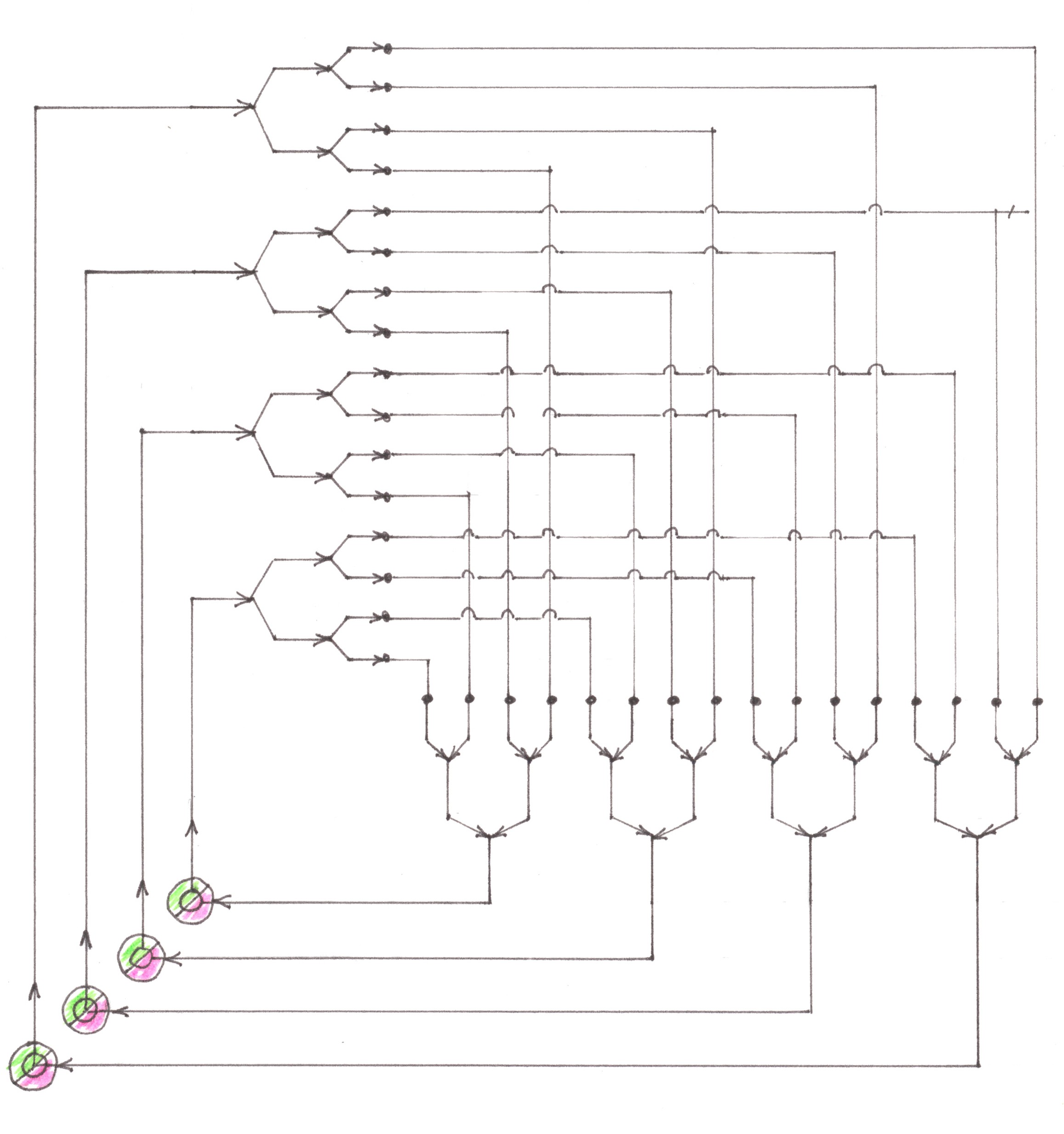
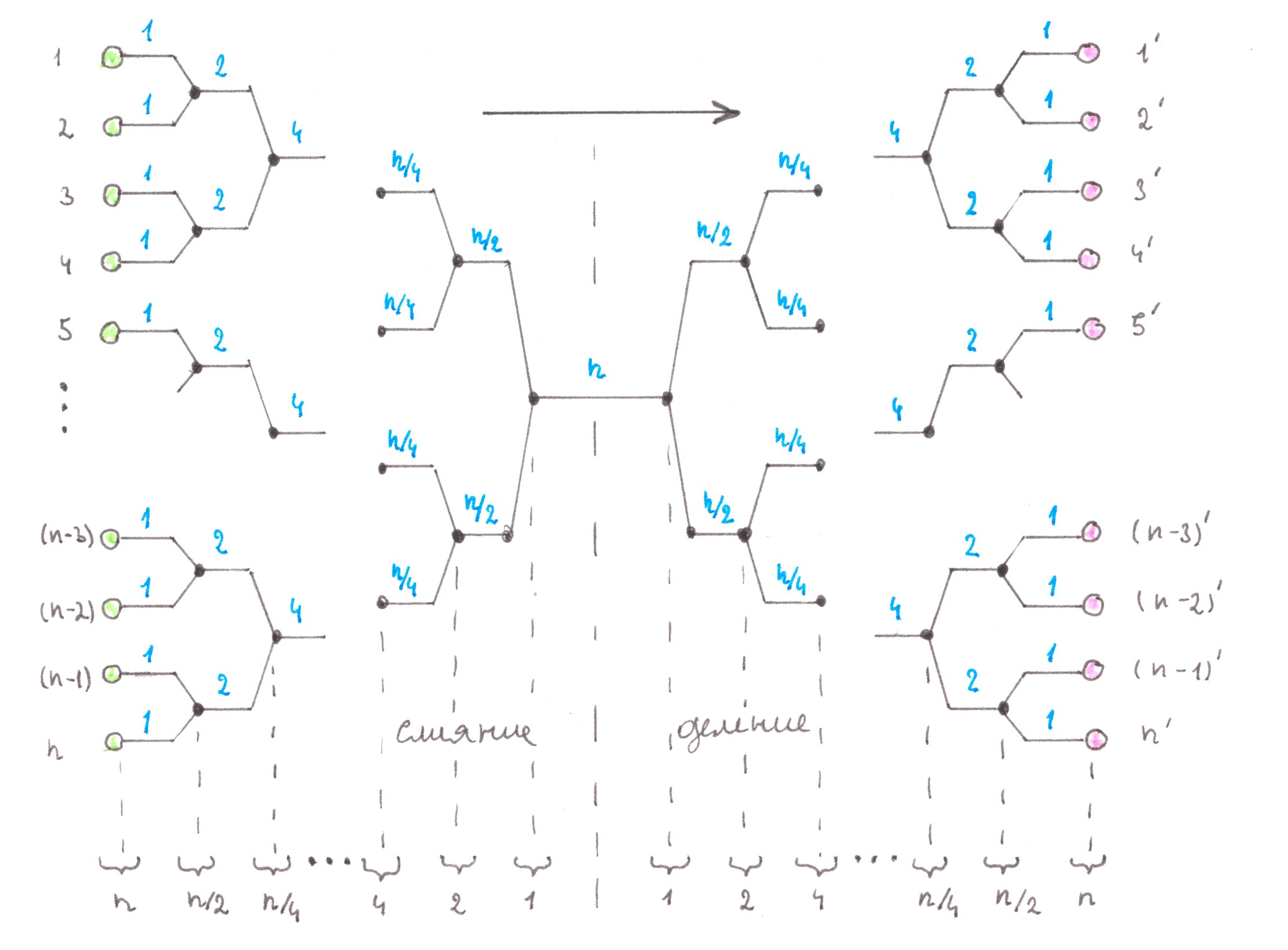
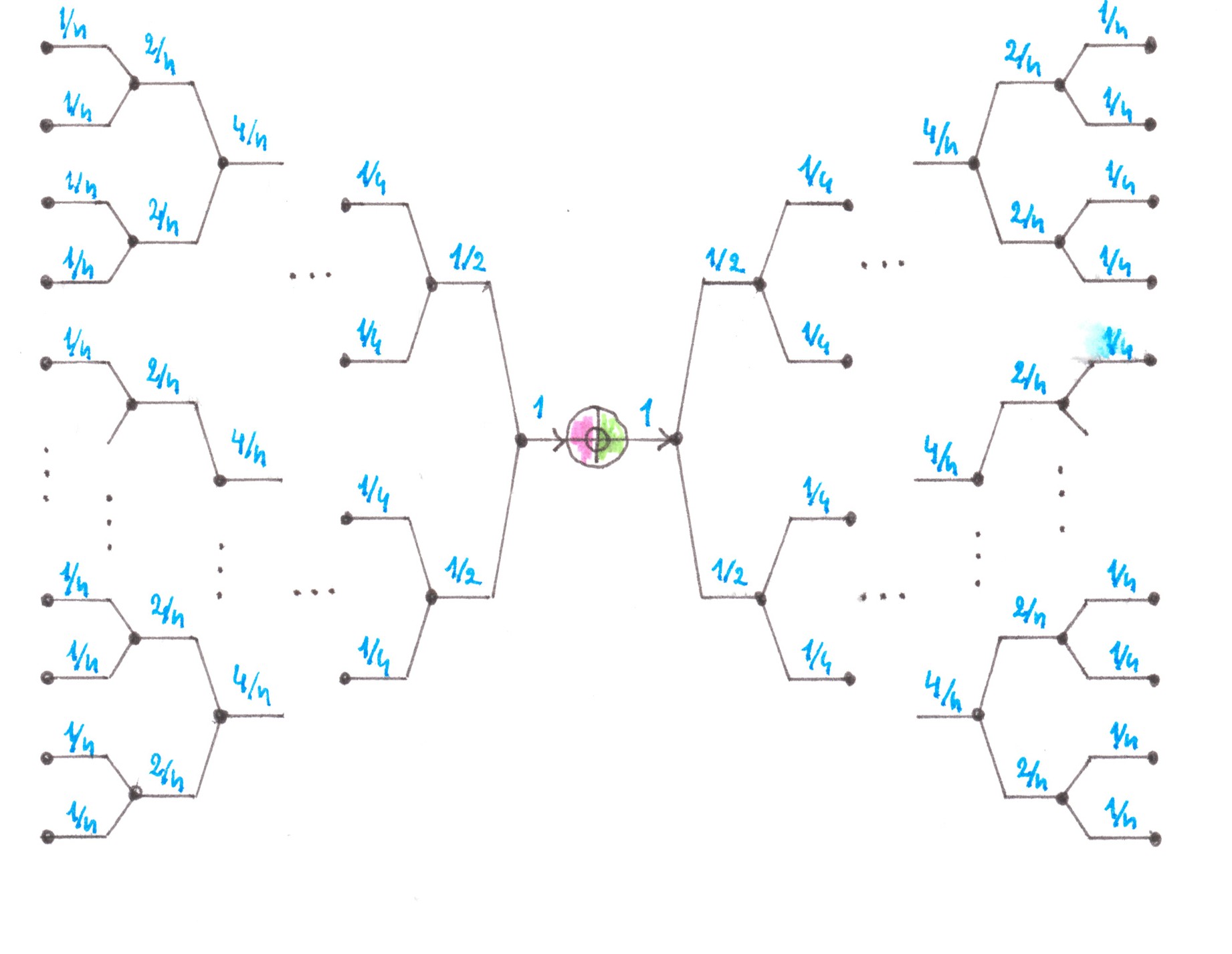
https://habr.com/en/post/473528/- Algorithms
- Mathematics
- Transport
- Urbanism
Chapter 2.
(
the link to Chapter 1)
The Art of Designing Road Networks
Transport problems of a city through the eyes of a Computer Scientist
If I were recommended an article with the title “The Art of Designing Road Networks,” I would immediately ask how many road networks were built with the participation of its author. I must admit, my professional activity was far from road construction and was recently associated with the design of microprocessors where I, among other responsibilities, was engaged in the resource consumption of data switching. At that time my table stood just opposite the panoramic window which opened up a beautiful view of the long section of the Volgograd Highway and part of the Third Transport Ring with their endless traffic jams from morning to evening, from horizon to horizon. One day, I had a sudden shock of recognition: “The complexities of the data switching process that I struggle with on a chip may be similar to the difficulties the cars face as they flow through the labyrinth of road network”.
Probably, this view from the outside and the application of methods that were not traditional for the area in question gave me a chance to understand the cause of traffic jams and make recommendations on how to overcome the problem in practice.
So, what is the novelty of the approach?
Historically, the main purpose of roads is considered to be the opportunity they provide to travel long distances fast (between Rome and the provinces). Such a judgment is justified when it comes to the federal-level intercity highway network: the cities that they connect look like small rare dots on the atlas, and most of the cars traveling between these cities pass their way without turning anywhere.
However, as soon as we turn over several pages and open a detailed map of a large city, the picture changes immediately: the number of addresses where the journey can be started or ended reaches approximately ten thousand, all of them are quite densely spread and relatively small in size. At the same time, hundreds of thousands of cars can be in motion on the streets of such a city at once, moreover, the goal of each of them is not just to fill already empty roads, but to move a person or cargo from a point with a specific address X to a point with a specific address Y. All together, this means that the urban transport system must be adapted to effectively solve the problem of multiple concurrent addressing. Thus, the functions of the urban transport system become even more similar to the telephone or computer network than the intercity road network.
Considering the road network as a switching circuit for a hardware developer or engineer in the field of information transfer technologies is a completely natural way to talk about a problem, but among people involved in research on transport problems, this view is, to my knowledge, new.
The theory of signal switching is a narrow engineering science and it alone, of course, is not enough to plan a separate street, road junction or predict the behaviour of a traffic stream on a straight, isolated section of a highway. Fortunately, the issues listed above are well researched today, and the methods developed to solve them have already successfully come into practice. The theory of switching, in turn, allows the architect to mitigate the risk, in which the city comes into a state of transport collapse despite the fact that all the elements of the road network are perfectly executed. This risk exists because performing multiple concurrent addressing is a resource- and time-consuming task, the key to an effective solution of which is not in the width of the streets and the convenience of transport interchanges, but in the competent choice of which particular switching scheme the proposed road network will implement.
From this research, for example, you will find out why the “arterial” type of transport networks, which are still often used in modern cities, are “bad” and together with the growth of the population will necessarily lead to traffic jams. Another interesting result, which is in good agreement with the observations, explains why the expansion of roads alone, if before all the traffic jams occurred exclusively in the vicinity of the interchanges, is unlikely to somehow improve the situation even if the number of cars in the city remains the same.
When I wrote this article, it was crucial for me that it was understandable to the most ordinary architect, could be useful through his work. I tried to introduce the reader into switching issues in a simple language, to develop criteria for assessing how well a particular road network will cope with the task of concurrent addressing, and using model examples I showed how to use this knowledge in practice.
The article is intended for a wide circle of readers who are slightly familiar with the university-wide course in mathematics, the theory of algorithms and are ready to devote 1 to 5 days to it.
Separation and merger of car flows
It is an obvious observation for many drivers that traffic difficulties arise mainly in those parts of the road where cars for some reason are forced to change lanes. Examples include road forks, narrowings, areas adjacent to highway exits and access roads, sections of highways where some lanes are blocked by an accident or roadworks.
In this section, an attempt will be made to give a quantitative description of the processes occurring in such cases, and we will start by understanding how cars switch lanes.
Two strategies to switch to an adjacent traffic lane
The traffic along a highway has a natural unevenness: someone prefers to drive a little faster, someone a little slower, between some cars the distance decreases and becomes hardly comfortable for driving, while between the others it increases so much that it allows cars to fit in there from adjacent lanes. The appearance of such gaps in the flow of the adjacent lane directly on the side of the random driver may be frequent or not very. If, at the moment when he needs to make a manoeuver, there is no gap, the driver can resort to at least two behavioural strategies:
Strategy 1
Several suitable gaps may simply be located close to the driver's location. If the movement is dense enough, then it’s unlikely that the driver will be able to add speed and catch the necessary gap, but by slowing down a bit the driver would let the neighbouring stream overtake the car so that to become equal with the gap that was originally behind — it would be not a big trouble. The costs of this strategy are obvious: the driver himself and the cars driving behind in his lane lose some time due to the need to reduce speed.
Strategy 2
In order to wait, you need to have patience and have the necessary amount of time for this. An alternative may be an attempt to perform the necessary manoeuver «here» and «now.» According to this idea, the driver gives a sign to the cars behind him of the lane to which he is going to move. Those, in turn, in response to his signal should slow down a bit and “let the cars moving in front of them to go forward”, thereby creating the gap of the necessary size in their flow. The time costs in this case are distributed between the cars of the lane, onto which the driver eventually switches.
In real life, both strategies are involved at the same time: at first, the driver slows down, waiting for a relatively large gap in the stream of the adjacent lane, and only after that, they give a signal to the cars moving in it about their intention to make a switching manoeuver.
Undoubtedly, access roads, highway exits and narrowings are not the only reason for the switching between lanes, which is worth remembering when designing roads. The ability of cars with higher speeds to overtake unhurried traffic is necessary in order to prevent the situation on the highway when it degrades to one large queue crawling at the speed of the slowest tractor. Nevertheless, the problem of coexistence of vehicles moving on a road at different speeds has a slightly different nature and can be separated from the issues in question, since the overtaking process and respective switching between lanes are not forced for the driver. If the driver does not hasten, according to the probability theory, a convenient opportunity to perform a manoeuver will be given to the driver naturally and for this he does not need to disturb the movement of other drivers.
The cost of a single switching
The behaviour of drivers in reality can be very complicated, but it is primarily crucial for us that the result obtained within model conditions remains plausible: each forced switching between lanes imposes a time penalty on traffic participants.
Let's now evaluate how the amount of lost time depends on the density of traffic on the road.
We will consider the movement along each lane as a separate stream. Trying to stay at a comfortable distance from cars on the same lane, drivers thereby reserve a road stretch with a certain characteristic length
d in the stream. Let
ρ cars fall in a stream per unit length. We agree to call the flow density small, or to say that
ρ is small if the product
ρ ×
d is much less than 1.
At the moment when the driver realises the need to move to the next row, the probability that a road stretch with the length
d, which the driver was going to occupy, will be not free, at small
ρ, will be approximately proportional to
ρ itself. If the described event really takes place, then two cars competing for a place will experience in total, as a result of the manoeuvers, some delay in the average constant value
δ.
Assuming
ρ is small, we can neglect the probability that their actions at this moment will affect the movement of other cars. Thus, when
ρ is small, the time loss from one switching will be
α⋅ρ, where the coefficient
α is an empirically measurable quantity depending on culture, weather, speed limits (and so on), but remaining approximately constant in this particular time and for this city as a whole.
Loss intensity rate on a road stretch before the exit
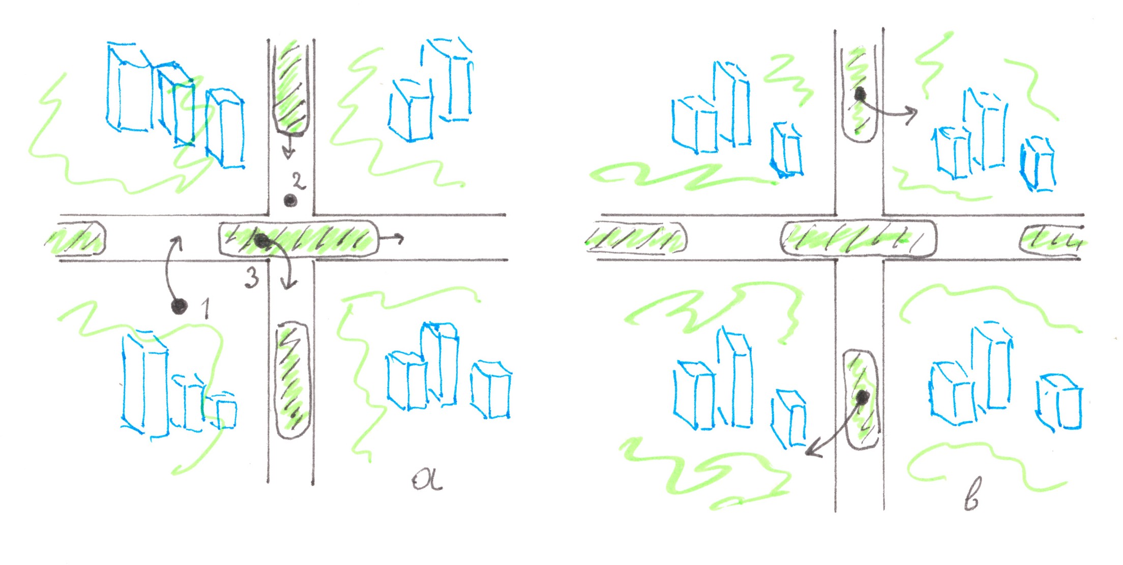
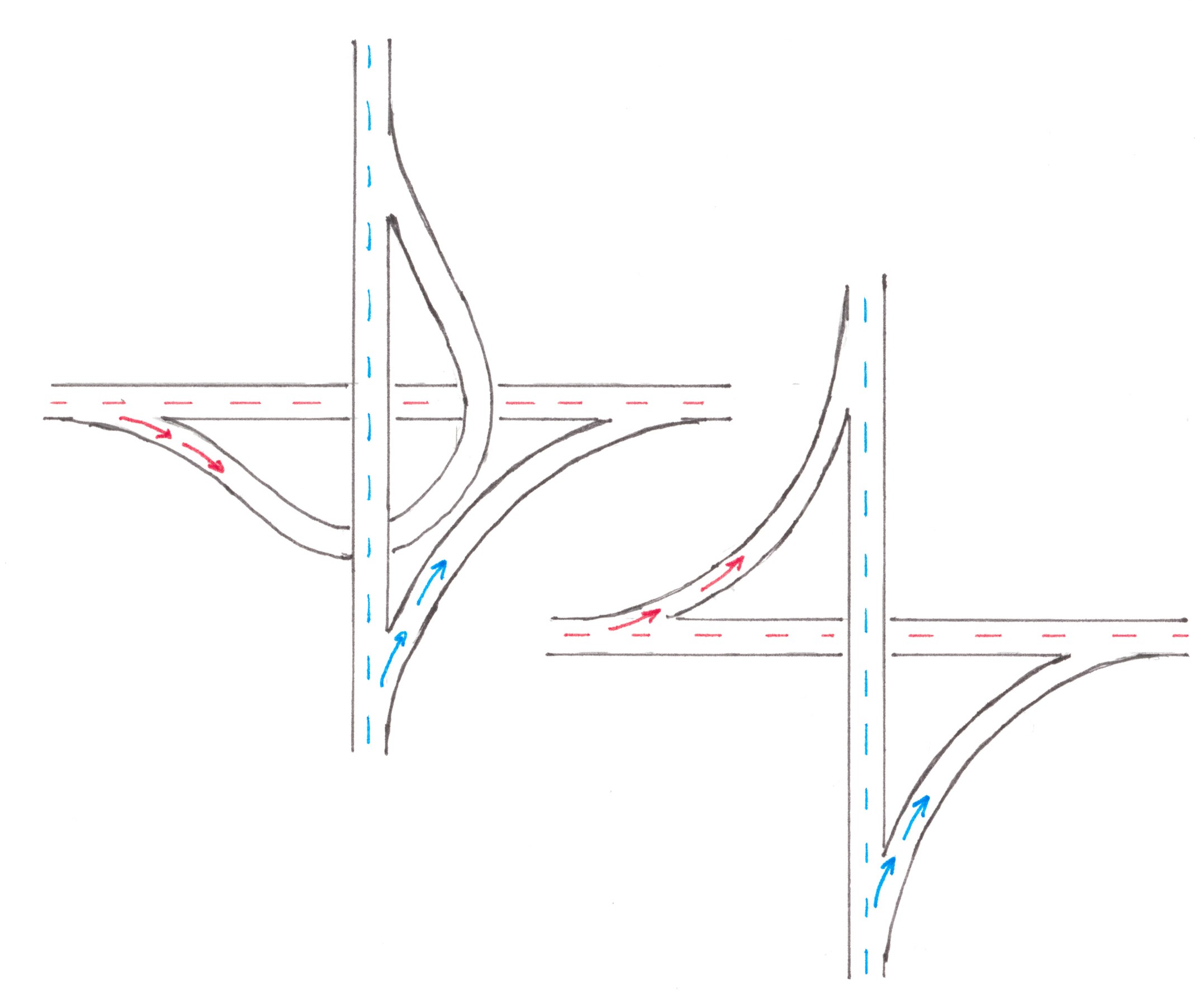
The cars heading for the exit, before they get to the ramp (Chart 2), have to, sometimes even several times, switch to the adjacent row on the right. Each such manoeuver disturbs the flow, and as a result, the average speed in the section before the exit is noticeably lower than in the “transit” (deprived of the exits, entrances and forks) sections of the highway.
Chart 2
To pass some part of the way at a lower speed — represents for drivers (and their passengers) an additional amount of time spent on the trip. In other words, the area of the highway adjacent to the exit is a constant generator of time losses.
Let's suppose that the average car speed
ν and the flow density
ρ at the frontal boundary of this stretch are the same for all lanes.
Moreover, let's suppose that the density
ρ and the flow rate
q heading for the exit (the average number of cars falling onto the ramp per unit time) are simultaneously small, and
s is the number of lanes on the highway. To get to the exit, the driver will make 1 to
s switching manoeuvers. If the flow density on the ramp is much lower than
ρ, then only the last manoeuver will be for the driver practically “for free”, while the rest will in any case cause losses of
α⋅ρ. On average, you will have to perform (0 + 1 + 2 +… +
s — 1) /
s = (
s — 1) / 2 “expensive” manoeuvers.
Given the difficulties caused by all cars heading for the exit, we can create the formula for the intensity of time losses:
Iout =
q ⋅ αρ ⋅ (
s − 1)/2 = (
α/2
ν)
⋅ q ⋅ (
sρν)
⋅ (1 − 1/
s)
The value
p = (
sρν) is nothing more than the flow rate of all the cars moving along the highway in the direction in question (the average number of cars passing by a bus stop per unit time). The last remark gives us the opportunity to rewrite the formula for
I a more symmetrical form:
Iout = (
α/2
ν)
⋅ pq ⋅ (1 − 1/
s)
Loss intensity rate at the adjoining section of the access road
The situation arising on the highway behind the section where the access road connects with it largely repeats the situation on the section before the exit, although there are some differences. Let a small flow of cars of power
q through the lateral ramp pours in the main traffic of the highway (Chart 3).
рис. 3
The ramp has only a finite length, so all newly arriving cars should be switched to the right edge lane of the highway. As a result, the traffic density in the right edge lane1 is locally higher than the average on the road, that's why some drivers in it decide to switch to a less busy adjacent lane on the left, which, in turn, leads to a local increase in density already on the second lane. This process of switching between lanes will continue until the flow density is leveled out across the entire width of the highway. Assuming the average speed
ν to be the same for all
n lanes, we can expect that, upon completion of the switching processes, the flow power in each of them will increase by exactly (1/
s)⋅
q.
To see how much such switching will cost to drivers, we at first calculate the power of all switching flows. The flow from the ramp to the first lane of the highway we already know: it is equal to
q. In order to equate the increase in the first lane power to (1/
s)⋅
q, the flow from the first lane into the second one should be (1 − 1 /
s)⋅
q, from the second into the third = (1 − 2 /
s)⋅
q, from the
k-th to the (
k + 1)th = (1 −
k/
s)⋅
q. According to the last formula, the capacity of the switching flow to the left edge lane will be (1 − (
s − 1)/
s)⋅
q = (1/
s)⋅
q, as commanded by common sense.
Since we know the time penalty of a single switching and the power of all switching flows, we can now calculate the total intensity of the losses generated by them:
Iin =
αρ⋅q +
αρ⋅(1 − 1/
s)
⋅q +
αρ⋅(1 − 2/
s)
⋅q +... +
αρ⋅(1/
s)
⋅q =
αρq (1 + 2 +... +
s)/
s =
αρq (
s + 1)/2 =
(
α/2
ν)
⋅ q ⋅ (
sρν)
⋅ (1 + 1/
s).
Remembering again that
sρν is the power
p of the flow of all cars along the highway, we obtain the cost formula in its final form:
Iin = (
α/2
ν)
⋅ pq ⋅ (1 + 1/
s).
Loss intensity rate at the symmetrical fork
In the previous paragraphs, we found losses from the interaction of flows, one of which was necessarily large, and the other was necessarily small. In order to demonstrate an approach to solving problems when the capacities of both flows are comparable in power, let us consider another extreme: a fork in which both branch directions are equally popular for drivers (Chart 4).
Chart 4
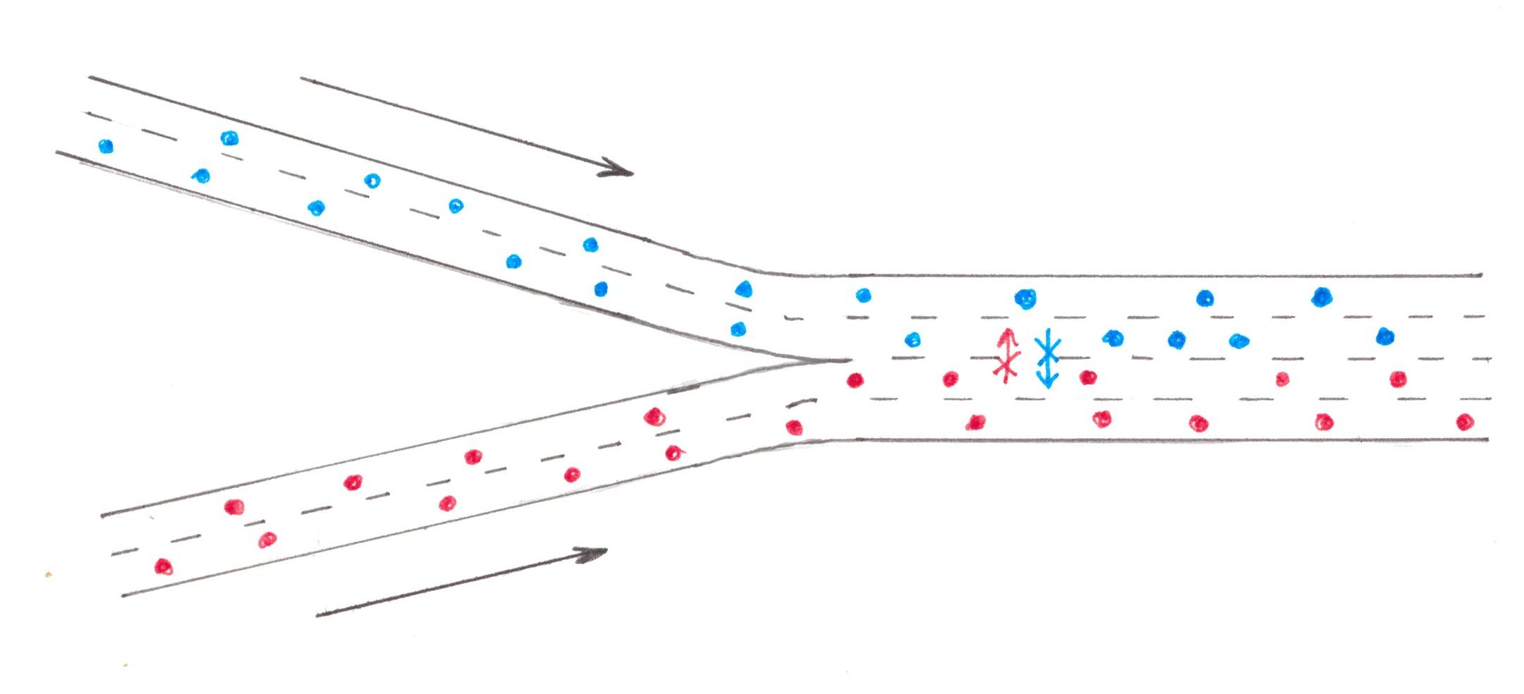
For convenience, cars going to the right on the fork will be called “blue”, and cars leaving to the left — “red”. Initially, cars of both «colours» move mixed, dispersed between all 2
s lanes of the highway. As they approach the fork, the red cars begin to drift slowly towards the left
n lanes, and the blue ones toward the
s right: there are switching flows in the two directions between adjacent lanes. Unlike the access road example, these flows are no longer “relatively small”. By the way, only between the two central lanes there is a forced exchange of traffic, the intensity of which in any of the directions (from left to right, or from right to left) is equal to a quarter of the power of the entire stream moving along the highway. Fortunately, in this situation there is a good enough way to estimate the generated costs.
At first, we can note that the process of dividing cars into “red” and “blue” most likely begins long before the fork and proceeds slowly, therefore, on the one hand, it should have little effect on traffic density within a separate row, and on the other, make switching streams stretched over long distances, thereby giving the opportunity to represent each of them as a combination of a large number of streams of low power (Chart 5).
Chart 5
Since now we are talking about small flows, albeit in larger numbers, nothing prevents us from reducing the problem in question to already solved ones. We can mentally divide the highway in the center into two equal parts, and then connect them together with a larger number of single-lane jumper roads, allowing red cars to get to the left and blue cars to the right (Chart 6). Due to obvious symmetry, when calculating the generated losses, we can focus on car of any one colour, for example, blue, and in the end just double the result.
Chart 6
Let speed
ν and density
ρ be the same for all lanes and remain constant over the entire stretch where cars are separated by colours. In this case, the flow power of all cars moving along the highway will be:
p = 2
sρv.
Let
q1,
q2,...
qm denote the flows of blue cars moving along imaginary jumper roads to the right half of the motorway. Suppose that shortly before the separation section in each lane of the motorway, both colours are represented with equal proportions of 50%, which implies that in total
q1 +
q2 +... +
qm equals to
sρv/2, or in other words,
p/4.
Losses generated by the flow
qidue to its smallness, we can calculate by the formula:
Ii =
Iout +
Iin = (
α/2
ν)
⋅(
p/2)
⋅qi(1 − 1/
s) + (
α/2
ν)
⋅(
p/2)
⋅qi(1 + 1/
s) = (
α /2
ν)
pqi
Summing up the last formula over all
i, we find the losses generated only by the blue cars:
Iblue = (
α/2
ν)
⋅p⋅(
q1 +
q2 +... +
qm) = (
α/2
ν)
p2/4.
The total losses, as already mentioned, will be twice as high and amount to:
Idiv = (
α/2
ν)
p2/2.
Analysis of the obtained formulae
If we divide the intensity
I, that is the amount of time totally lost by the participants per second, by the lateral flow
q, which by definition is equal to the number of cars connecting or leaving the highway in one second, we will get the average losses caused by one such car:
iin =
Iin/
q = (
α/2
ν)
⋅ p ⋅ (1 + 1/
s)
iout =
Iout/
q = (
α/2
ν)
⋅ p ⋅ (1 − 1/
s)
Perhaps the most important thing in these formulae is the direct proportionality between the power flow of cars on the highway
p and the unit costs
i. Everything looks as if a car seeking to join, or vice versa — to leave the main flow, thereby causing constant disturbance to every driver nearby.
The second, interesting and very unexpected observation concerns the extremely weak effect on the intensity of the generated losses in the number of lanes near the highway directly next to the junction. As you can see, looking at the formula for
Iout, the exit is generally the most time-efficient for a single-lane road (
s = 1,
iout = 0 ), and the difficulties caused by the adjoining access road for a three-lane and six-lane highway differ by only
100%
⋅ [(1 + 1/3) − (1 + 1/6)] / (1 + 1/3) = 12,5%.
If we consider that every car that has ever joined the traffic on the highway will eventually have to leave it, then it seems quite legitimate to use a unified value instead of
iin и
iout when calculating interchange losses
iav = (
iin +
iin)/2 = (
α/2
ν)
⋅ p.
Despite the fact that the formula for
iav does not explicitly depend on the number of lanes, it must be remembered that its creating (see the assumptions for
Iin and
Iout) bases heavily on the assumption of low density of cars on the road, so it is unlikely to give satisfactory results when applied to too narrow highway with too much traffic.
Preliminary findings
In areas near junctions, traffic hindrances inevitably occur, taking time away from drivers, reducing the average speed, the latter leads to an increase in the density of cars and, as a consequence, the possible occurrence of traffic jams. The time losses associated with the separation and merger of car flows will be called switching losses.
Losses of a similar type are present one way or another in any switching scheme: be it a telephone or computer network, a multi-core microprocessor, or a mail delivery service.
When the driver joins, or, conversely, leaves the traffic on the highway, the switching costs incurred by his actions are proportional to the power of the flow of cars observed at that time on the highway.
To reduce switching losses throughout the city, it is necessary to carefully consider the road network implemented in it at the design stage. A bit later we will analyse this task in detail, but some obvious recommendations can be listed now:
- switching losses are proportional to the flow power on the highway — it is not necessary to enlarge the roads without the need, two small highways are twice as good as one big one;
- switching losses are proportional to the power of the side flows — it is worth designing the network so that the driver has to turn as few times as possible during his journey;
- mutual disturbance caused by the drivers of the main and side flows should be less on a citywide scale if we try to prevent merger of routes that overlap only in a short section of the road.
Economic prerequisites for the existence of cities.
A city model with 'random access'2
(Note 2: the term is taken from the RAM concept and means random by probability and even by time consumption.)
Perhaps the first stage of any project to design (or re-design) the city transport system is to try to determine what kind of switching the city really needs now and how its needs will change in the future.
Such an analysis can be carried out if we first divide the city into not too large, but not too small areas, and then for each pair of such zones indicate what approximate number of trips to one side or the other is needed by their inhabitants at one or another time of the day. By placing the predictions made in a matrix, you will thereby receive a migration needs matrix of the city residents.
Exactly for this matrix, we should search a network that allows drivers and passengers to spend as little time as possible on a separate trip, requiring from the city authorities as little resources as possible for the network realisation.
When it comes to existing cities, it is important here not to make a mistake and not to replace the number of trips that people really need with the number of trips that have historically been established under the influence of some obstacles or difficulties at the time of the design work. Probably, the transport network of Berlin “before” and “after” the fall of the separation wall can serve as the most striking illustration of what has been said.
This section will mainly deal with humanitarian issues in which I am not a specialist, but I think that discussing them as an amateur is nevertheless more correct than simply avoiding the problem.
In order to better represent the migration needs of the population, it is worth starting with the fundamental question: “What are cities for and what is their useful function?”
Let's try to answer it not as ordinary residents of cities (and villages), but from the perspective of the person responsible for the process of urbanisation in some large and developed state. From this point of view, it is no longer important what historical motives once made so many people crowded into a tiny piece of land, or the reasons why they continue to do it now, it is crucial — what economic effect is made by the cities of one size or another and by what mechanisms this effect is achieved.
In my opinion, the main reason for the existence of large cities is, on the one hand, the opportunity for technology firms to find employees of rare professions, and on the other hand, the opportunity for people who have mastered rare professions to sell their services to companies interested in them on competitive terms. In a small (non-specialised) city, the production of many goods and services is either simply impossible, or puts the technology companies and their employees in the position of mutual hostages, without giving either one or the other any alternatives.
For example, take the not-so-rare profession of a school literature teacher. According to statistics, the need for them is approximately 1 teacher per 1000 people. In a regular school, 3-4 tutors teach literature. The choice of a job for a literature teacher can be called competitive if there are at least 4-5 secondary schools in the city, which, in terms of population, corresponds to about 15 thousand people.
Apparently, people with an engineering specialisation feel comfortable on the labour market in cities with a population of at least 100 thousand. Of course, there are also such professions, the demand for which appears only in cities with more than one million people, however the existence of multi-million cities does not make any economic sense to me.
After all the above-mentioned, two hypotheses look quite reasonable (the validity of which, however, does not affect the truth of the main contents of the article):
- the average adult has a need to travel most frequently over distances that capture 4-5 of the most promising jobs for them;
- for a significant part of the population that represents the rare and most economically valuable professions, the distance of the most frequent trips may well be comparable with the radius of their city.
As an enhanced reflection of hypotheses 1 and 2, in my examples I will often use the model of the city with 'random access', assuming that the power of the flows of required travel is the same between any two quarters of it, or, in other words, in all cells of the migration needs matrix there are the same positive number. If you randomly look at the records of trips made in such a city during the day, then for the next marked trip all quarters will have the same probability of being whether the start or finish of such trip, and no relationship between the position of the 'initial' and 'final' quarters should be observed.
Road networks with the simplest topology
Let's try to apply the ideas described in the previous paragraphs to some types of city plans taken from life.
Linear city
The first large settlements were originated predominantly along the coast, in areas of a thin strip of land between the sea and the cliffs, or along the paths of busy roads, so in the process of growth they acquired narrow elongated borders. Many of these settlements have survived to our days, retaining their elongated shape and turning into modern cities (please see the illustration below).
 (an excluded area of Rio de Janeiro, the author is unknown)
Often in such a city there is only one wide road around which it is built. Suppose that each quarter (zone of territorial division) generates a stream of travels with power 1, the number of all such quarters equals to
n, and the city itself follows the 'random access' migration model.
Chart 7
Let us try to find for the parameters listed above how the average travel time and the required road area change with increasing
n.
So, let all the quarters have the same shape and size, and their number multiplies by
λ (lambda) times. It's obvious that
- the length of the main road increases by a factor of λ.
Due to the accepted model of 'random access', 50% of the journeys that started in the right half of the city will end in its left half (the opposite will be correct too), therefore, with an increase in the number of quarters by a factor of
λ, the power of the flow passing through the middle of the city will also multiply by
λ times. Similar discussions with the same inference will be true if, instead of the middle, we take any point dividing the city in a given ratio (1:3, 2:5), which implies that
- the power of the flow along the main road increases by a factor of λ;
- the number of lanes of the main road required in each section multiplies by λ times.
More or less obvious that the average length of the trip, and with it
- the net travel time spent to cover the distance increases by a factor of λ.
All that remains to calculate is the number of times the time lost due to switching costs in one trip will increase. A lateral flow with power 1 enters into and comes out of each quarter, which together generate time losses with intensity:
I =
Iin +
Iout = (
α/2
ν)
p⋅2,
where
p is the power of the flow on the main road. We already know that the number of quarters and the flow power on the main road increases by a factor of
λ, therefore, the total time losses generated by the network multiply by
λ2 раз. On the other hand, the number of trips generated by the network, between which as a result all these losses are allocated, increases by a factor of
λ, that's why
- the net travel time lost due to switching costs increases by a factor of λ.
Let's exhibit all the results in one table:
Linear topology
The number of address points (quarters) with power 1 ........................
n
Total road area......................................................................................O(
n2)
Net travel time,
spent to cover the distance...................................................................O(
n)
Net travel time,
lost due to switching costs.....................................................................O(
n)
Number of switching nodes...................................................................O(
n)
Number of switching nodes, given the power of the side flows.............O(
n)
Notation used '
y = O(
x)' means that the parameters
x and
y are functionally dependent, and when
x grows without limit, the ratio
x/
y tends to a finite, different from zero, number.
Cellular city
The second, fairly common planning method is to arrange the quarters in the form of a rectangular matrix, similar to how portioned pieces are placed in a chocolate bar.
We agree to call such cities 'cellular'.".
 (Los Angeles, photo: Slava Stepanov)
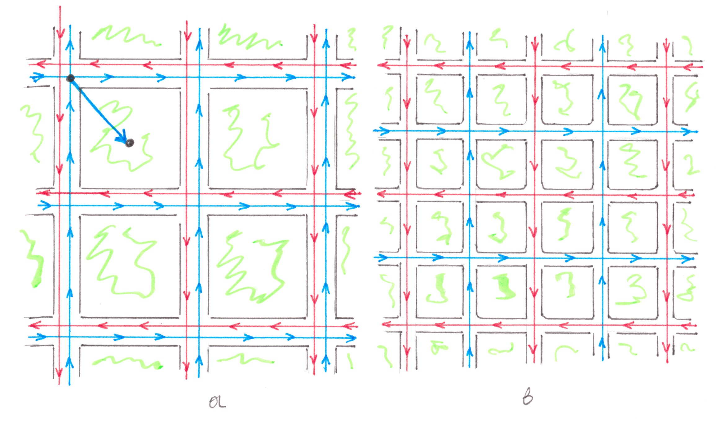
Chart 8 shows a pattern of a cellular city which consists of
n (taking into account the 'halves') quarters, forming together a regular square. The quarters are separated from each other by a total of √
n roads, conditionally stretching from west to east, and √
n roads stretching from south to north. In total, these roads form √
n×√
n crossings, each of which can be implemented either as a traffic light intersection or through road bridges / overpasses.
Chart 8
Regardless of whether there is one-way or two-way traffic, any journey from point A to point B in a cellular city can be realised along a route involving no more than two streets and no more than one turn at an intersection.
Assuming that, as in the previous example, each quarter generates a stream of travels with power 1, and the migration needs of the population follow the 'random access' model, we can calculate, now for a cellular city, the laws by which the average travel time and the resource intensity of road network construction will change with increasing quantity of quarters.
If the number of quarters increases by a factor of
λ, then:
- the area of the city multiplies by λ times, and its linear dimensions while maintaining the proportions — by √λ,
- the average travel distance and the net time to cover it, being proportional to the linear dimensions, multiply by √λ times,
- the number of streets and the number of quarters adjacent to one given street multiply by √λ times,
- the power of the traffic flow, being proportional to the number of quarters with which the flow is 'in contact' (an explanation of this term will be given later), multiplies by √λ times,
- the required area of all roads grows as (number of streets) × (length of one street) × (power of street flow) = √λ⋅√λ⋅√λ = λ√λ
Lateral flows are divided into those that go from or towards the quarters and those that turn from one street to another at intersections. The power of first flows, according to the conditions, always remain equal to unity. Through the second ones, almost all traffic is moving, coming or leaving the highway, if we take into account that there are much more quarters in the city than quarters on one given street. As a result, the change in the power of the second flows can be estimated by the formula (change in the power of the flow) / (increase in the number of intersections on a particular street) = √
λ / √
λ = 1. Equality of the last ratio to the constant suggests that these flows do not significantly change with an increase in the number of quarters, therefore, the increase in switching costs generated by the network as a whole will be: (increase in the total number of quarters + intersections) × (change in the value of the flow on a single street) =
λ√
λ. Since the power of the migration flow generated by all quarters increased by a factor of
λ, then
- net travel time lost due to switching costs increases by a factor of √λ
Let's exhibit all the results in one table:
Cellular topology
The number of address points (quarters) with power 1.....................
n
Total road area...................................................................................O(
n√
n)
Net travel time,
spent to cover the distance................................................................O(√
n)
Net travel time,
lost due to switching costs.................................................................O(√
n)
Number of switching nodes................................................................O(
n)
Number of switching nodes, given the power of the side flows..........O(
n)
Comparing the linear and cellular networks with each other, it is difficult not to notice that the increase in the resource intensity required for construction and the time spent on one trip, with the growth of the city, is much faster for the first network than for the second one. For example, a cellular city consisting of 100 quarters requires 10 times less asphalt, and traveling through it on average requires 10 times less time compared with a linear city of the same size. Therefore, it makes sense to use road networks with linear topology only in very small towns.
If for a while we forget about the existence of switching costs, then cellular topology can be considered an ideal way to design road networks, since it gives an asymptotically optimal O-estimate for both the average trip length and the required road area. Indeed, for any more or less 'compact' location of the city (with random access), the length of the trip will grow no slower than the square root of the area of the city, which is in turn usually directly proportional to the population. As a result, we get all the same O (√
n).
The fact that a typical route in a cellular city runs along a 'corner' rather than a straight line, in principle, implies the opportunity to look for the best ways to plan cities, but the savings in the amount of 20% (that’s the maximum we can win if cars learn to travel through walls) are unlikely someday will force architects to abandon the rectangular arrangement of streets and roads.
The lowest possible limit of the network building (and maintaining) costs can be obtained by remembering that each car reserves a part of the lane for its movement. As a result, the total area of roads is proportional to the product of the average travel time (average trip length) and the number of cars in the city: O(√
n)×O(
n) = O(
n√
n) (compare with the table for a cellular city).
If we talk about the amount of time that is lost in travel due to switching costs, then surprisingly its relation to the amount of time to cover the distance does not asymptotically depend on the number of quarters in either cellular or linear city (O(√
n)/O(√
n) = O(1), O(
n)/O(
n) = O(1) ). In other words, the percentage of time lost in travel due to switching, in both big and small cities, will be the same. From this we can conclude that, if there were no serious problems with switching costs in a small city (we can suggest they amounted to 10-20%), then in a big city they still should not be observed, and if they were, then they would remain to exist, no matter how the city grew and enlarged.
Since we do not know which of the alternatives is true (or rather, we know that problems with traffic in big cities do exist), it is worth trying to improve the topology of a cellular city so that the switching costs in it decrease at least by a factor of some constant times.
Useful examples of unrealistic networks
Let's test if cellular topology follows the recommendations that we have developed by analysing the switching of flows on the highway.
1) Do not enlarge roads without the need.
— Yes. Traffic is distributed over many roads (compare with a linear city).
2) Avoid designing the network where the driver has to turn a large number of times in one trip.
— Yes. Any trip will most likely be carried out along a route requiring only one turn on the streets.
3) Try to prevent merger of routes that overlap only in a short section of the road.
— Here, perhaps, there is something to work on. Despite the minimum number of turns per trip, the route as part of the main highway flow passes through a large number of switching nodes (O(
n)), in each of which valuable time is wasted.
The last remark motivates to investigate the following question: “What is the minimum of the average number of switching nodes through which a journey must pass through a road network connecting
n quarters?”
The task of searching for such a network makes sense, of course, only on condition that the number of flows combined or divided by any switching node is preliminarily limited from above by a certain fixed value. Otherwise, you can always present a road network with
n address points and a single mega-junction.
 (the author is unknown)
It is much easier to investigate the real problem if it was previously possible to reveal at least part of the patterns using some simple, even if not at all realistic, model examples. Following this logic, we will temporarily forget about the geometrical limitations of road construction and the need of travelers to cover distances, focusing all our attention on how abstract networks solve the parallel addressing problem. Regarding the switching nodes, we will assume for now that each of them either divides the flow into two parts (the division node), or combines two flows into one.
Chart 9
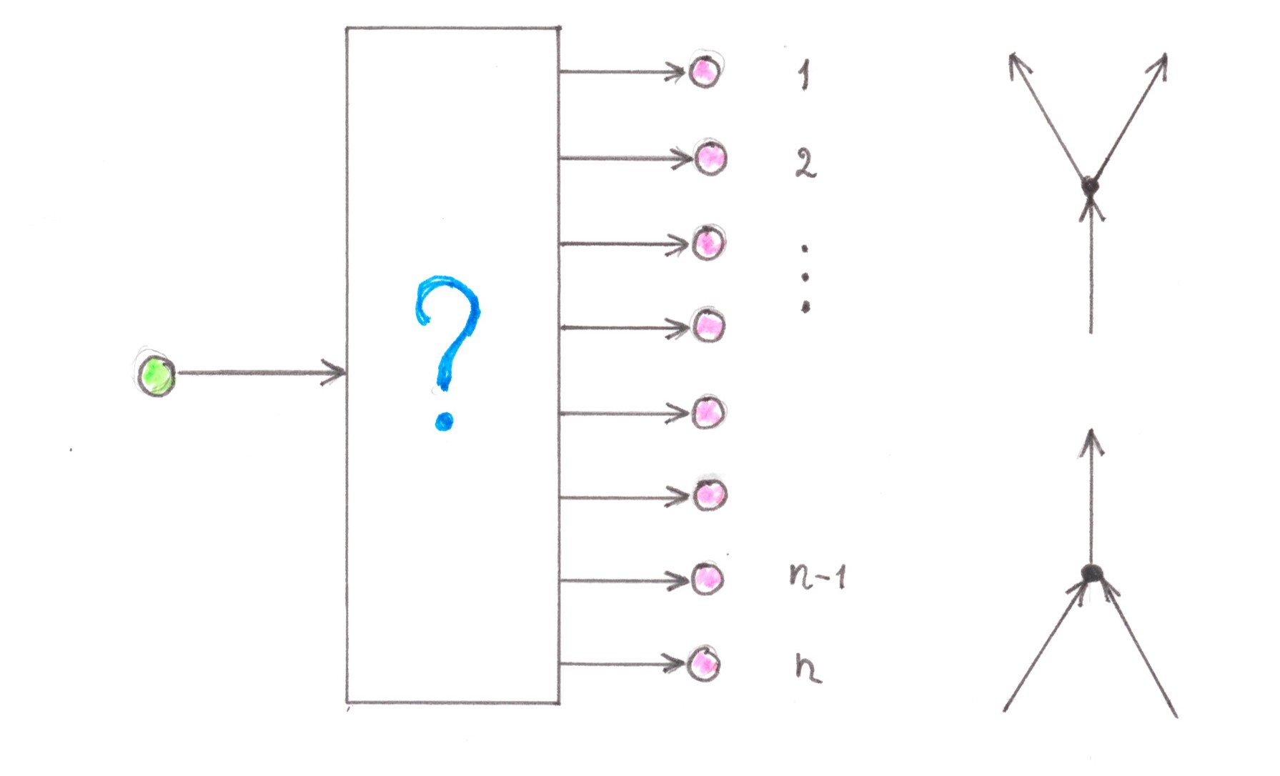
Address tree
Let there be one
start address point, where all travels, without exception, begin, and another
n finish address points at which they end with equal probability (Chart 9).
It is required to build a transport network that allows the driver to go through as few switching nodes as possible.
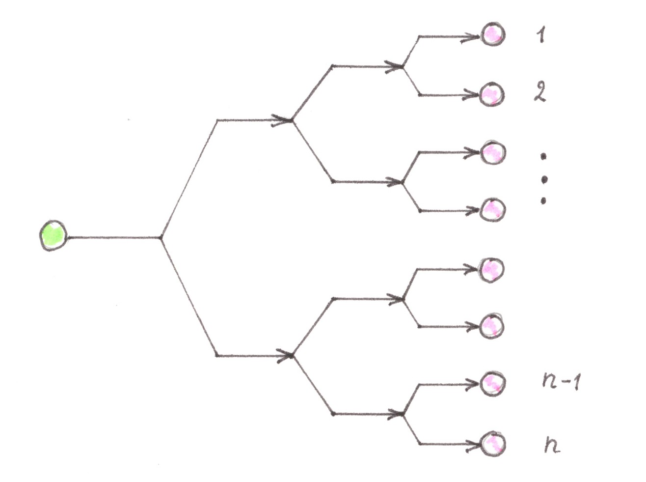
The obvious (for programmers) solution, which suggests itself here, is to use a balanced binary tree, at the same time we need to place a single start point at the top of the tree, and place the remaining
n finish points one in each of its leaves (Chart 10). The network constructed in the described way will be called as the direct Address tree.
Chart 10
Changing the directions of all flows in the direct Address tree to the opposite, we thereby obtain the
reverse Address tree, the purpose of which is to connect
n start points with a single finish point.
In cases where
n is a power of two, any route inside the Address tree passes exactly through log
2n switching nodes, which is undoubtedly (asymptotically) less than the same indicator for a network with cellular (O(√
n) ), or linear (O(
n) ) topology.
Two simplest types of logarithmic networks
Using 'tree-like' networks as building blocks, it is not difficult to generalise the previous solution to the case when there are
k start points. There are two easy ways to do this.
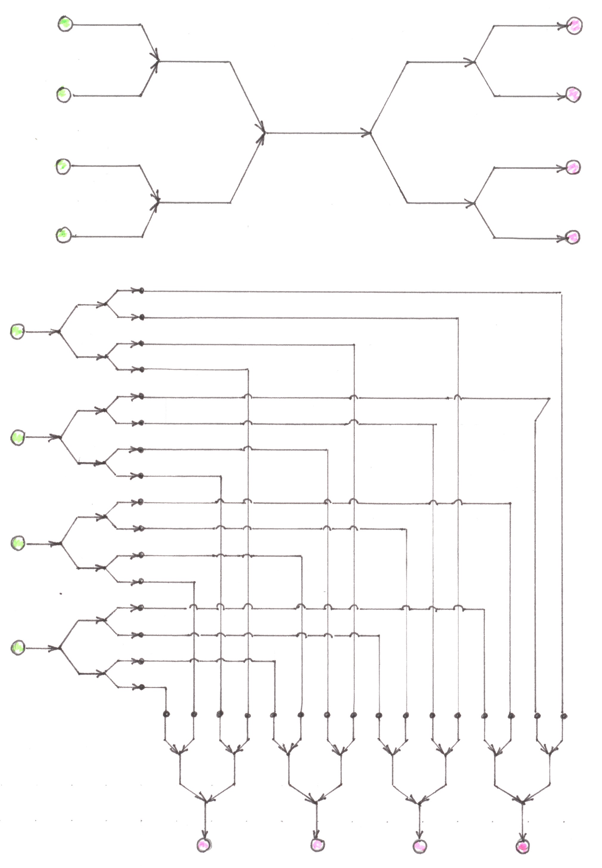
The first way is to use the reverse Address tree to first collect the routes of all the trips into one common stream, and then, using the direct Address tree, divide this stream into sub-flows addressing to its destination (Chart 11, top scheme).
Chart 11
If
k and
n are powers of two, then, in the end, any route passes exactly through the log
2k + log
2n узлов коммутации. witching nodes. We agree to refer to the networks designed according to the algorithm just described as (one-way)
Logarithmic networks with preliminary merging.
The second way to solve the same problem can be realised by reversing in the first solution the order of the merging and division operations. Its implementation can be described as follows: for each start point we create a unique set of imaginary duplicates of all the finish points, and after that, we connect it to these duplicates (no longer imaginary) with a direct Address tree.
To complete the network design, it remains only to connect now each finish point with its
k imaginary duplicates by applying the reverse Address tree (Chart 11, bottom scheme).
Whenever n and k are powers of two, the number of switching nodes along any route within the newly built network will again be equal to log
2k + log
2n.We agree to refer to such networks as (one-way)
Logarithmic networks with preliminary division.
Conversion of one-way networks into symmetric ones
Generally we refer to any network as one-way if the address points connected by it are divided strictly into start and finish points. By default, for one-way networks, it will be assumed that it provides at least one route of possible travel from any start point to any finish point.
Besides a lifelong journey, it is difficult to find examples where some address points would serve as the start of a route only, and others would only be its end. We will bring our reasoning closer to reality if we also include networks in which any two address points are connected by routes in both directions. We agree to refer to such networks as symmetric.
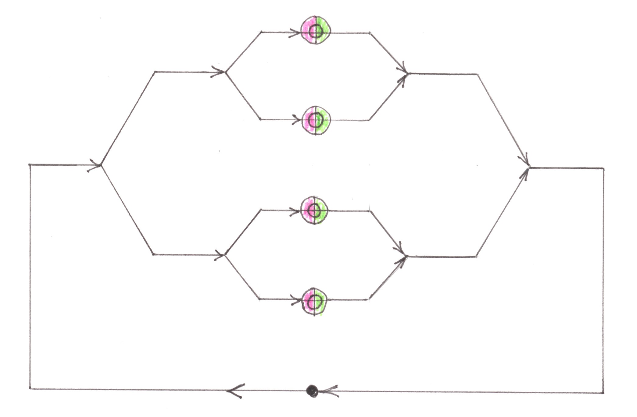
In fact, there is no ideological gap between one-way and symmetric networks: each symmetric network can also be used as a one-way network, and each one-way network, initially connecting an equal number of start and finish points, can be transformed into a symmetric one (Chart 12).
Chart 12
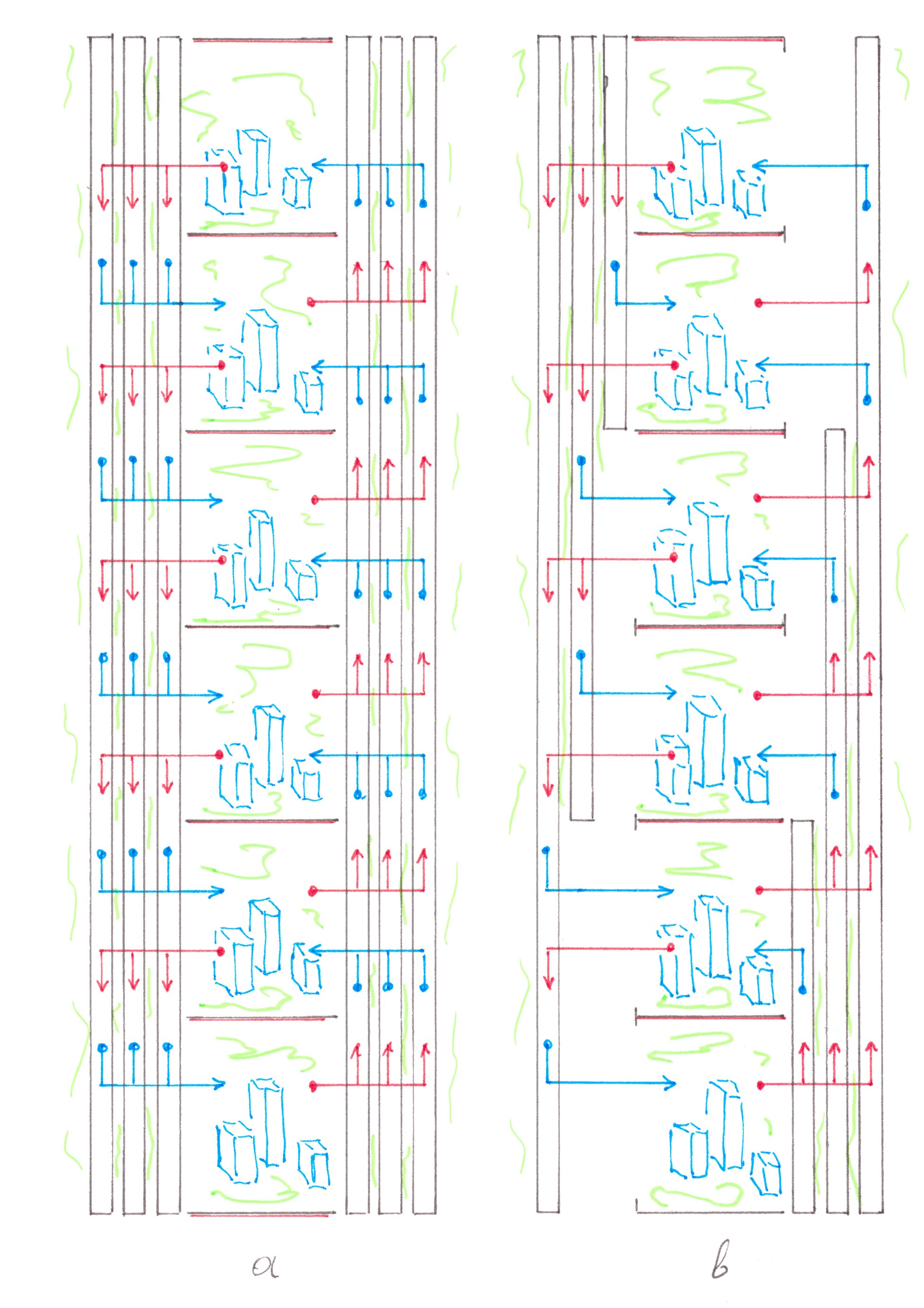
Charts 13a and 13b show the 'symmetric' forms of the Logarithmic network with preliminary merging and the Logarithmic network with preliminary division. Their examples prove the fundamental possibility of connecting n quarters by such a type of network, within which the number of switching nodes during any trip will be proportional to the logarithm of the number of quarters in the city.
Chart 13 a
Chart 13 b
Accurate lower limit estimate
A wide variety of networks has already been accumulated so far, each of which include own function describing dependency of the average number of switching nodes along the journey on the number of address points in the city. Nevertheless, we still do not know how small this number can be in principle for a given number of quarters. The lower limit estimate can be obtained using the information approach.
Actually, let some road network connect
n address points to each other, and the migration needs of the population are such that any trip, no matter where it started, has an equal chance of ending anywhere in the city.
To solve the problem in question, we will generate an auxiliary informational message, following this recipe: for a long period of time, we will collect records of all the trips that have a fixed start point, and randomly write down the addresses where these trips ended. The resulting message will be a random sequence which consists of the names of
n address points of the city.
One way to transmit this message to Mars is firstly to encode all the names into binary words of the same length, thereby turning the original message into a sequence of 0s and 1s, and secondly to send the resulting sequence through a digital communication channel. Since for distinguishable coding of the set of
n names binary words of log
2n length are required, the length of the digital message will be:
(number of records)×log
2n characters.
The most interesting thing is that according to information theory, regardless of the encoding algorithm used, it is simply impossible to transmit the same message with a smaller number of binary characters.
An alternative to directly transmitting the encoded names of the finish points can be a method in which it is indicated for each trip in what possible direction the route turned at the next fork. According to our assumptions, all the forks in the network can only have two branches, therefore, to indicate the direction in each case, exactly 1 bit is required. For anyone who has a map of the city and knows the starting point, the chain of bits will be enough to trace each route and restore the original sequence of their destinations. If the average number of forks (division nodes) visited during one trip is
x, then the length of the binary message with the new encoding method will be: (number of records)×
x.
As there was said earlier, the new encoding method cannot be more efficient than the direct binary address transfer method, therefore: (number of records)×
x ≥ (number of records)×log
2n, that's why:
x ≥ log
2n.
Although the last inequality was initially deduced for a group of trips that had a common fixed start point, it turned out to be independent of the specific choice of this point. That's why we can extend the result to all trips in the city at once, thereby obtaining the first part of the estimate in question:
P1) Provided that each new trip has equal probability of finishing at any of the
n address points of the city, the average number of division nodes per route cannot be less than log
2n.
Mentally turning the clock back, we can convert each finish point of the trip into the start point, and each binary node of the division of the network — the binary node of the merging. This little trick allows us to automatically obtain from P1 the second, missing part of the estimate:
P2) Provided that each completed trip would have equal chances to start at any of the
n address points of the city, the average number of merging nodes per route cannot be less than log
2n.
If we recall the existence of a logarithmic network with preliminary merging and a logarithmic network with preliminary division, then we immediately get two examples of networks that are optimal in terms of the number of switching nodes, which, on average, is visited inside them during one trip. Let's see if this quality helps reduce the intensity of the generated switching losses.
Switching costs in Logarithmic networks
If we compare the networks with preliminary merging and preliminary division, the first one looks much more attractive because of its simplicity. Unfortunately, this simplicity also has a reverse side to the coin: combining all routes into one stream contradicts
i1 recommendation, thereby potentially causing large time losses. The network with preliminary division seems to meet the requirements
i1 —
i3, however, judging from Chart 13b, it tends to rapidly increase the number of road limbs and switching nodes used. The latter quality may make networks of this type too expensive for practical use.
We will analyse these questions in more detail. To begin with, we agree that the city follows the migration model with 'random access', and the flow generated by any of its address points has a power 1.
Losses in the networks with preliminary merging
In Chart 14 you can see a diagram of flows arising from the above-mentioned conditions within the network with preliminary merging.
Chart 14
It seemed to me convenient to depict the network itself in its one-way form, implying that each start and finish points, signed with the same numbers in the Chart, actually mean the same address point in the city.
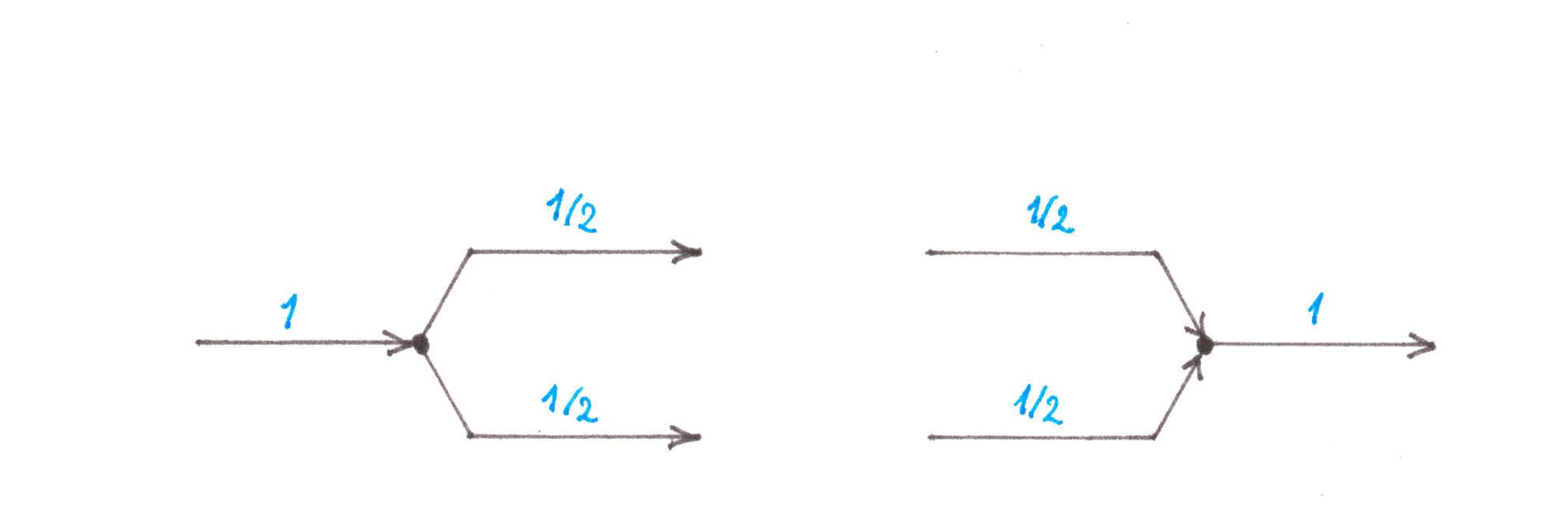
Based on the diagram, we can calculate the switching costs intensity generated in the network. Let's start from the left half, where through the reverse Address tree, all routes are gathered in one flow. Each switching node in this part of the network represents the place where two one-way highways merge into one (Chart 15).
Chart 15
If initially each of the roads is efficiently loaded, then after their merging, there is no need to reduce the number of lanes, as a result, there should not be any respective switching costs.
Let's suppose that a flow with power 1 is already sufficient to effectively load the road along at least two lanes. In this case, we will come to a rather unexpected conclusion: the merging of car flows inside the Logarithmic network with preliminary merging occurs absolutely 'for free', without causing any time losses.
Calculation of the costs that arise in the right half is not much more difficult. This part of the network is a direct Address tree, each node of which is a symmetrical fork we have already studied. When the incoming flow with power
p, the intensity of the losses arising at the fork is (
α/2
ν)
⋅p2/2. The power of the flow entering the root fork is:
n, therefore, the intensity of losses in the root node is: (
α/2
ν)
⋅n2/2. In each next generation of the Address tree, the number of forks doubles, and the power of the incoming flow is halved. As a result, the formula of the losses inside the whole tree will take the form:
It_div1 = (
α/2
ν)
⋅(1/2)
⋅[
n2 + 2 (
n/2)
2 + 4 (
n/4)
2 +… + (
n/2)
⋅2
2 ] =
(
α/2
ν)
⋅(
n/2)
2 [ 1 + 1/2 + 1/4 +… + 2/
n ] ≈ (
α/2
ν)
⋅n2
Since the power of the flow of trips generated jointly by all address points is
n, the time costs per trip are on average (
α/2
ν)
⋅n, thereby showing a linear dependence on the size of the city.
When it comes to abstract networks, it is difficult to give any meaningful estimate of the area of the roads they use. As an alternative measure of structural complexity, the total power of all side flows can be calculated. As planned, the resulting value should reflect the resource intensity of building of all the interchanges required by the network. I can’t say that in practice this method will always have a good interpretation, but some approximate idea of the amount of work ahead will probably be obtained.
Inside the Logarithmic network with preliminary merging, lateral flows exist only in the direct Address tree, and their total power for each generation of nodes is the same:
n/2. In total, there are log
2n of generations of nodes in the tree, thus a new method for assessing complexity gives an estimate of complexity: O(
n log
2n ).
Logarithmic networks with preliminary merging
The number of address points with power 1....................................................
n
Average travel time
lost due to switching costs:
asymptotics......................................................................................................O(
n )
exact value.......................................................................................................(
α/2
ν )
⋅n
Number of switching nodes..............................................................................O(
n )
Number of switching nodes, given the power of the side flows........................O(
n log
2n )
Losses in the networks with preliminary division
We now turn to the analysis of the Logarithmic network with preliminary division, again assuming that the network is used to connect the address points with power 1 in the city with 'random access'.
Chart 16 shows a fragment of it consisting of one address point along with the direct and reverse Address trees adjacent to this point.
Chart 16
First of all, we can estimate the intensity of the switching losses generated by the fragment.
The costs incurred during division of the flows can be found by the following equation
It_div1 = (
α/2
ν)
⋅n2, which was deduced for the direct Address tree in the previous example, 1 instead of
n. Indeed, the direct Address trees in Charts 16 and 14 have the same depth and involve the flows similar in power (note: similarity means the ability to get one set of values by multiplying the values from another set by some fixed number, to illustrate, the similarity between triangles by their sides). Due to the quadratic relationship between the value of the switching costs that occur at a single fork and the power of its incoming flow, a simultaneous decrease in all flows by
n times will reduce losses in the entire tree by
n2 times, therefore, instead of the old (
α/2
ν)
⋅n2, we obtain a value equal to:
It_div2 = (
α/2
ν).
We can now calculate the value of the costs in the left half of the fragment.
Due to the little value of the combined flows of the road inside the reverse Address tree, this time it would not be reasonable to build a road wider than two lanes. Merging under such conditions is no longer for free: in contrast to the previous example, there are narrowing areas on the highway (Chart 17), where switching costs will be necessarily occur.
рис. 17
Assuming that the driver is aware of the forthcoming narrowing in advance, we can assume that the process of switching from the dead end lane is slow, being stretched hundreds of metres along the highway. In this case, we have the right to resort to the trick that we used earlier to calculate the losses at the symmetrical fork — to divide the total migration flow
q into many small parts
qiand then interpret each of them as a side stream from the ramp. The losses generated by each such substream are calculated by the formula:
Ii = (
α/2
ν)
⋅ pqi ⋅ (1 + 1/
s), however, there are two subtleties here.
The first one is that cars will not migrate further than the next row.
In fact: the flows in the two central lanes, due to obvious symmetry, should always have approximately the same density, so drivers will not have much reason to cross the middle line. From the observation made, it can be inferred that in the formula for losses caused by partial lateral flow,
s is equal to 1.
As the cars leave the edge lanes, switching into two central lanes, the flow power inside the central lanes gradually increases, changing in each case from
P/2 to
P. Thus, the second subtlety is the significant dependence of
p on the number of substream
i, which makes us write:
not
Ii = (
α/2
ν)
⋅ pqi ⋅ (1 + 1/
s),
but:
Ii = (
α/2
ν)
p(
i)
⋅ qi ⋅ (1 + 1/
s).
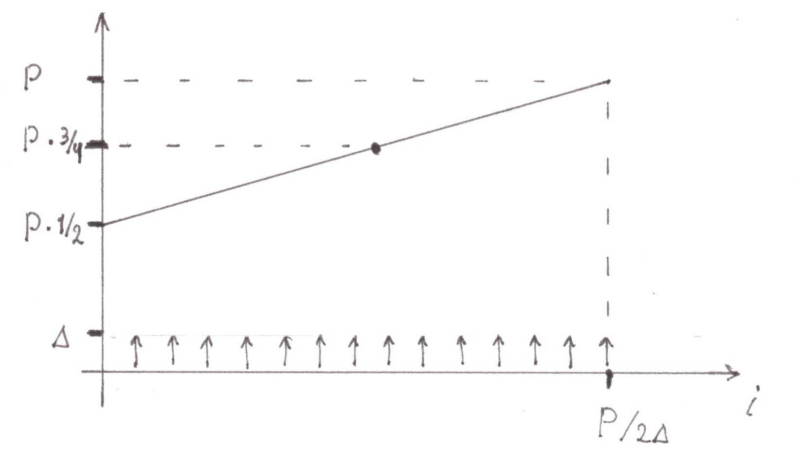
In the case when many small parts, into which the migration flow was divided, were all of equal size, the dependence
p(
i) is expressed by a linear graph (Chart 18)
Chart 18
To calculate the loss intensity rate, we must either resort to integration, or (this makes it possible to make a particularly simple form of an integrable function) take as
p(
i) the average value on the graph equal to 3
P/4. Since the total migration flow from the side of each edge lane is
P/2, the intensity of losses in a separate merger node will be:
Imerge = 2
⋅ (
α/2
ν)
⋅ (3
P/4)
⋅ (
P/2) =
= (
α/2
ν) 3
P2/4.
To find the time losses generated inside a fragment on the reverse Address tree, we can apply the formula for
Imerge to each of its nodes:
It_merge = (3/4)
⋅ (
α/2
ν) [ 1
⋅(1/2)
2 + 2
⋅(1/4)
2 + 4
⋅(1/8)
2 +… + (
n/2)
⋅(1/
n)
2 ] ≈
≈ (3/4)
⋅ (
α/2
ν) [ 1/4 + 1/8 + 1/16 +… ] =
= (3/8)
⋅ (
α/2
ν) [ 1/2 + 1/4 + 1/8 +… ] =
= (3/8)
⋅ (
α/2
ν).
The total costs arising within the fragment due to the merger and division of flows will be:
It_merge +
It_div2 = (
α/2
ν) [ 1 + 3/8 ] = 11/8 (
α/2
ν).
A logarithmic network with preliminary division contains only
n such fragments, and exactly
n flows with power 1 are generated by its address points, so the value we have just found is exactly equal to the switching losses per average trip.
In fact, it’s more important for us not even a specific number, which is equal to the specific switching costs, but the fact that these costs remain constant with increasing
n. The latter makes the Logarithmic network with preliminary division asymptotically the most economical with respect to switching losses among all the types of networks that we studied earlier.
Unfortunately, leadership is not free. Despite the vanishingly small value of the overwhelming number of flows, each Address tree included in the network contains about 2
n two-lane road limbs and approximately
n full-sized switching nodes. There are 2
n trees in the network, which meansO(
n2) limbs and nodes, which makes it not only the most economical in terms of time efficiency, but also the most expensive network to build, among all the examples considered.
As for the sum of the lateral flows, its value, as can be easily calculated, grows with the speed O(
nlog2
n) and in this case does not carry much meaning.
Logarithmic networks with preliminary division
The number of address points with power 1......................................................
n
Average travel time
lost due to switching costs:
asymptotics.........................................................................................................O(1)
exact value..........................................................................................................11/8 (
α/2
ν ).
Number of switching nodes.................................................................................O(
n2 )
Number of switching nodes, given the power of the side flows...........................O(
n log
2n )
Balanced logarithmic network
Exceptionally small switching losses and at the same time considerable resource consumption of the network construction, arising from applying of a logarithmic network with preliminary division, make us want to find some way to change its design so that the resource consumption would be significantly reduced whereas the switching costs would not increase substantially.
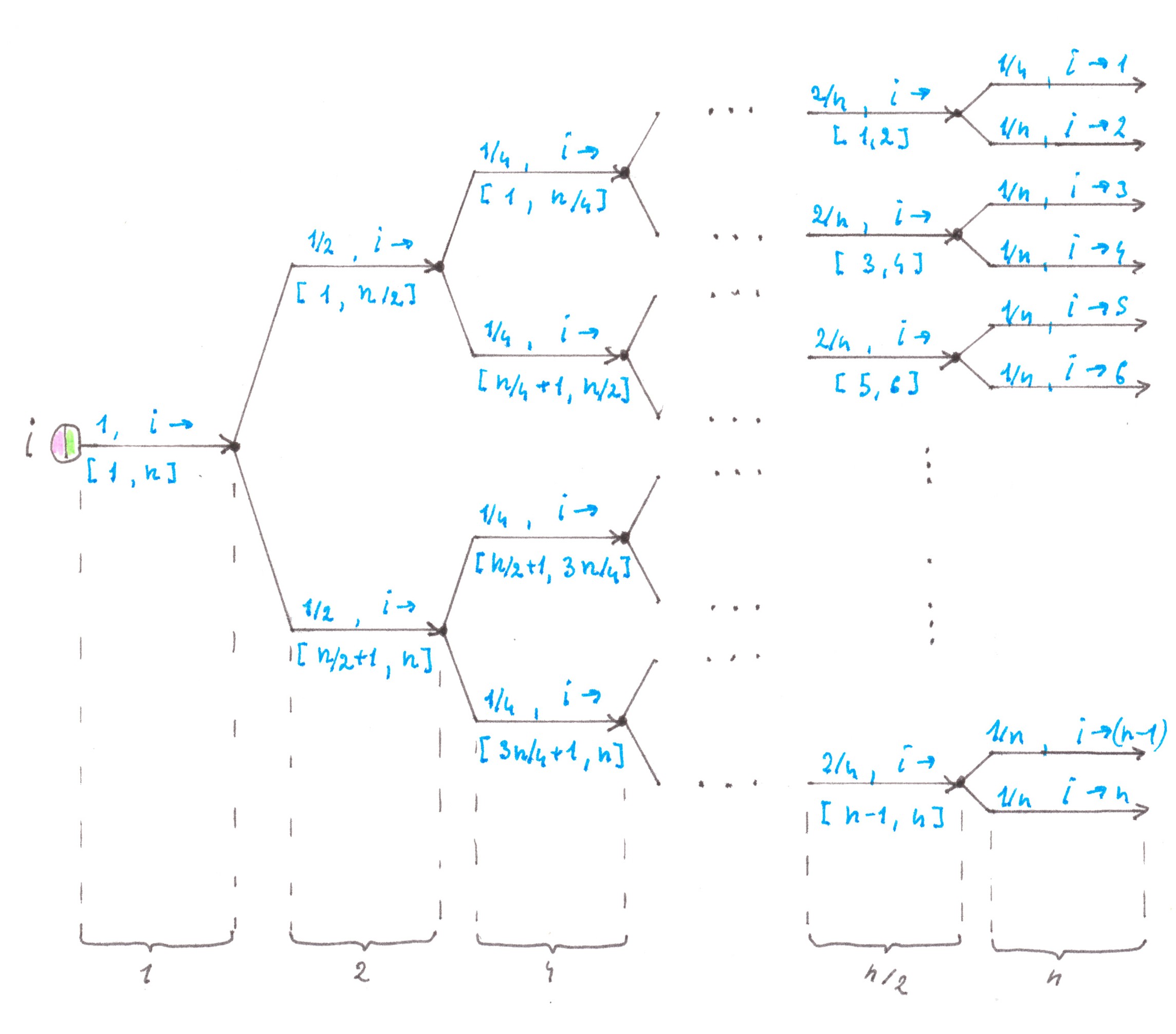
Obviously, the main culprit for an excessively large number of roads in the network is the extremely low efficiency of their use. The latter is clearly seen in Chart 19, which shows a detailed diagram of flows inside a direct Address tree adjacent to the ith address point.
Chart 19
In the chart, the number above the limb of the tree denotes the power of the flow passing along the limb, and the range below is the set of address points between which this flow will eventually be distributed. We assume that all the limbs presented in the chart are two-lane highways, the number of limbs in each generation of the tree is indicated at the bottom of the figure.
Upon careful consideration, you may notice that the rule by which the flow is divided in a particular node is determined solely by the position of this node inside the Address Tree and does not depend on the number of the address point that gave start to these trips.
If there are several flows addressed to the same set of points, and each of the flows is not powerful enough to fill the path allotted to it, then why don't we combine them together into one highway. In fact, this essentially simple idea makes it possible to build a good abstract network that generates relatively small switching losses and is economical in terms of the number of roads used.
Returning to the Address tree of the i-th point, we see that the flow entering into the root node is divided into two son flows with a capacity of 1/2 each. The first son flow consists of trips addressed to points from the range [1;
n/2], the second one consists of trips addressed to points from the range [(
n/2) + 1;
n].
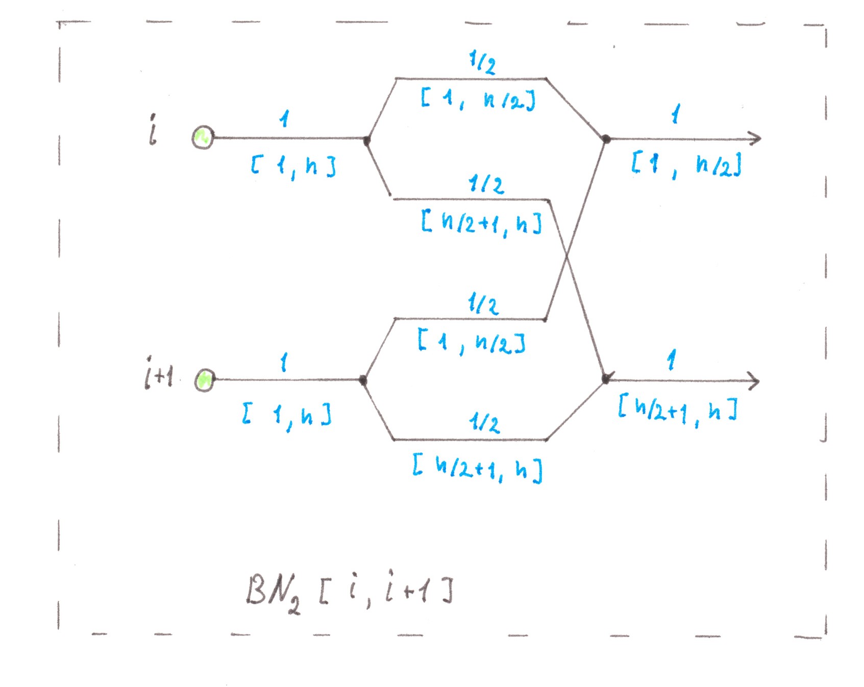
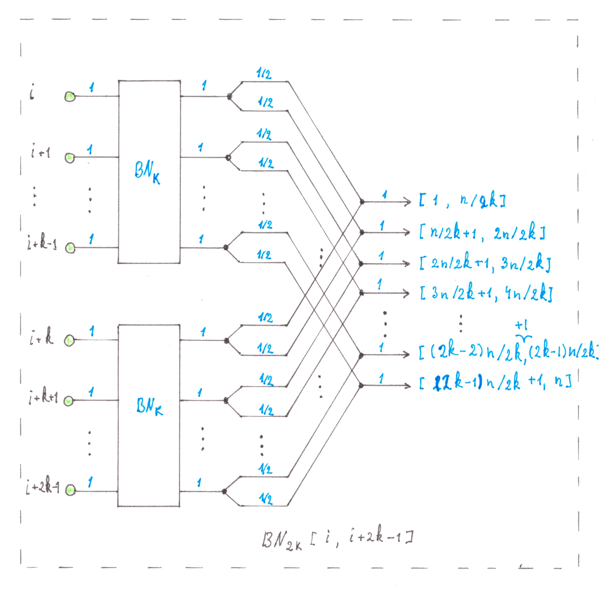
Following the idea outlined above, we combine the son flows of the same type at each odd point and the address point following it in order with an even number. This technique allows us for each selected pair of points to have, instead of four flows with a power of 1/2, only two flows with power 1 (Chart 20). We will name the obtained fragment of the future network as BN
2[ i; i +1].
Chart 20
f the son flows were not combined, but were still inside the Address tree, then in the next generation of nodes, each of them would again be divided into two parts, equal by power and by the size of the sets of the address points to which the trips are heading.
Why break the established tradition, because after the combining process we still have the same set of flow types as before, but with only fewer representatives of each type. To each of the output flows from BN
2[ i; i +1], we can apply exactly the same division rule that would apply to a flow of its type inside the Address tree.
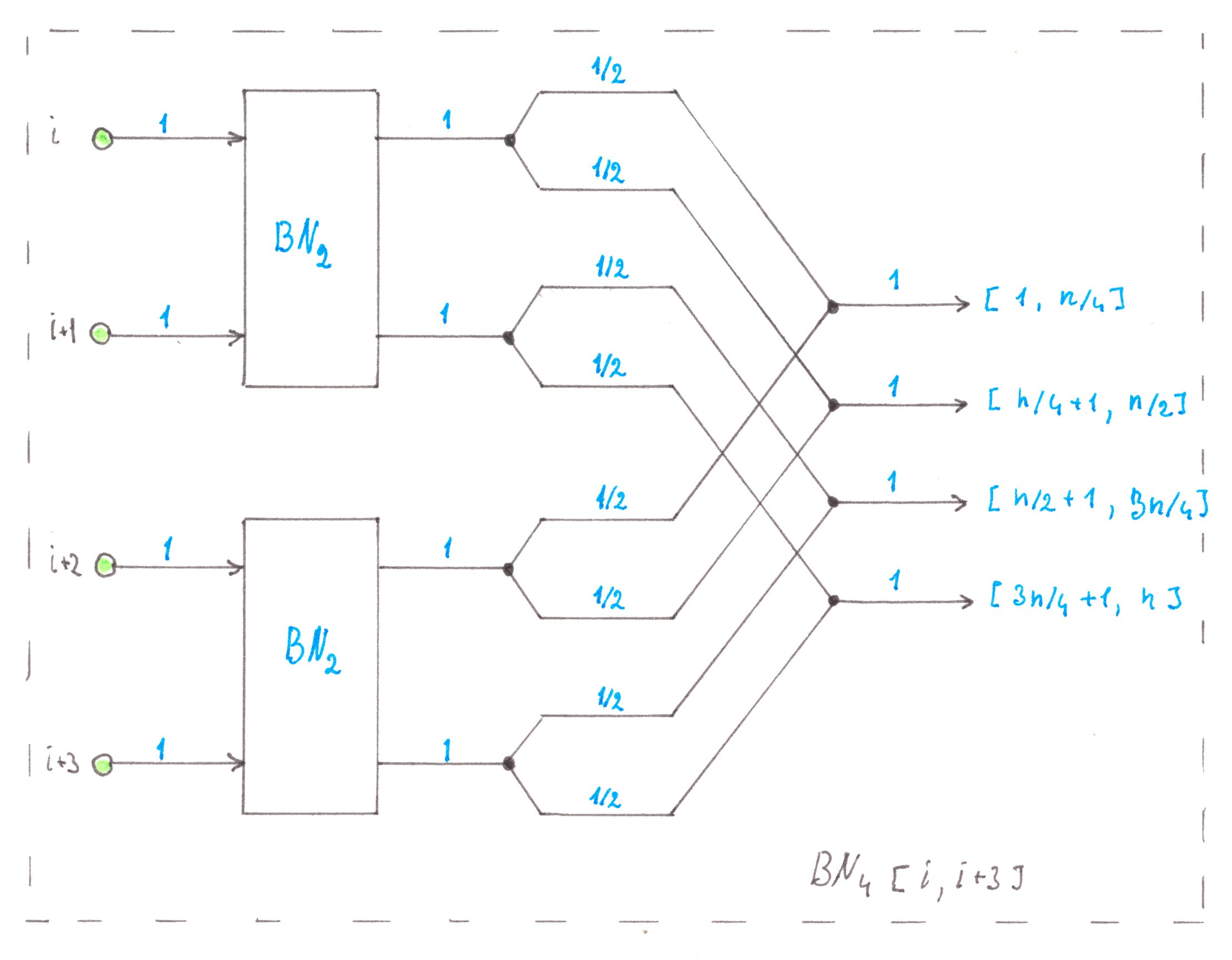
There is no reason for not repeating inductively the logical construction described above for combining-splitting of the same flows. Chart 21 shows a scheme for combining two fragments
BN
2 into one fragment of BN
4, on the other hand, Chart 22 shows the same algorithm in the general case.
Chart 21
Chart 22
In the end, the process of fragments' enlargement will be completed and lead us to the only element BN
n[ 1;
n ]. We will call it the Balanced logarithmic network (Chart 23).
Chart 23
Let us examine this network for the complexity and value of the generated switching losses.
Based on the inductive nature of the Balanced network designing, the number of switching nodes included in its structure can be described by the recurrent equation:
nodes( BN
k ) = 2
nodes( BN
k/2 ) + 2
k,
with the following limitation:
nodes( BN
1 ) = 0.
The solution to this system of equations is the function:
nodes( BN
n ) = 2
nlog
2n.
Since the designing of BN
n requires log
2n induction steps, each journey will go through log
2n division nodes and the same number of merging nodes, alternating between them on its way (Chart 24).
Chart 24
Losses generated within each division node:
(
α/2
ν )
⋅ (1)
2 /2.
Losses generated within each merging node:
(
α/2
ν )
⋅ 3
⋅ (1/2)
2 /4 = 3/16 (
α/2
ν ).
Considering that the number of both of them in the Balanced Network are
nlog
2n, we can get the exact value of the total switching losses:
11/16 (
α/2
ν )
nlog
2n,
which per one trip is:
11/16 (
α/2
ν ) log
2n
Balanced logarithmic network
The number of address points with power 1....................................................
n
Average travel time
lost due to switching costs:
asymptotics......................................................................................................O( log
2n )
exact value......................................................................................................11/16 (
α/2
ν ) log
2n
Number of switching nodes.............................................................................O(
n log
2n )
Number of switching nodes, given the power of the side flows.......................O(
n log
2n )
The figures obtained above allow us to consider the Balanced Network as a good compromise between the quantity of time losses introduced and the overall structural complexity. Its use as a road network of a real city is in principle possible, but hardly economically feasible. It seems to me that the area where the use of the Balanced Network can actually be of great benefit is large-scale information systems with strict requirements for the amount of signal delay, such as cellular communications, the Internet, distributed computing, and multiprocessor computers. For us, the greatest value of the Balanced Network is the method by which it was designed. A little later, using a modification of this method, we will be able to improve the networks of linear and cellular cities that are really crucial in practical terms.
Why historical cities are doomed to traffic jams
My statement may seem unexpected, but the answer to the question why naturally developing cities, usually suffer from traffic jams, was already found by us in the previous paragraphs. So what is the essence of it?
The fact is, many historical cities that survived after the era of medieval fortresses (for example, almost all the capitals of the “Old World”) inherited from this time the radial structure of the streets. Unfortunately (for their modern residents), a road network with a similar topology does not scale well: the dense arrangement of radial roads near the center is becoming too rare on the periphery. As a result, in the process of population growth, the streets that were initially located on the sidelines of the few roads leading to the fortress became larger and the streets that appeared on the periphery were short and did not acquire sufficient transit significance to grow in breadth. As a result, the road network that we see now in large historical cities most often refers to Arterial-type transport systems, and in our terminology, to the Logarithmic networks with (incomplete) preliminary merging.
 (Moscow roads, photo: Slava Stepanov)
If we talk about the length of the roads that a driver should drive along, the implementation of this type of network is not bad: the distance traveled often differs little from the straight line distance, and its average value in the city, as it should be for “decent” transport systems, grows at a rate of O(√
n). The trouble is that with the enlargement of the city at the Logarithmic network with preliminary merging, the switching costs generated by it increase too quickly: the amount of time for which, on average, the trip is extended because of them, depends on the number of people living in the city like O(
n). It is clear that starting from some
n, this time will prevail over the net time to overcome the distance, in other words, traffic jams will appear in the city.
Undoubtedly, the reorganisation of the transport system in large historical cities is a task that can be solved. However, it is important to understand that the construction of another one, two or five large transport arteries, albeit slightly improve the situation in the city, but will not eliminate the root cause of traffic jams. Apparently, the only way to overcome the drawbacks of the Logarithmic network with preliminary merging is to use another network. A good candidate here may be a network with cellular topology, within which the time to cover the distance is growing, at least, at the same rate as switching losses are growing.
 (night Berlin, photo: Vincent Laforet)
Perhaps that is why modern Berlin, although with large arterial highways, is already distinguished by a clearly visible cellular structure.
There are many interesting solutions in the world on how to make residents of historical cities more mobile, but the main prize in the struggle for transport accessibility should probably be given to the engineers of Barcelona.
 (Barcelona's updated road network, photo: Vincent Laforet)
A closer look at the networks of Linear and Cellular cities
After the methods of analysis were found and honed on abstract networks, now it is time to apply them to more realistic cases of cities with Linear and Cellular topology. In this section we will try to analyse in all details the features of their transport networks, establish the numerical value of the switching losses intensity rate, find how its value depends on the size of the quarters, and discuss possible variations and improvements.
Linear city
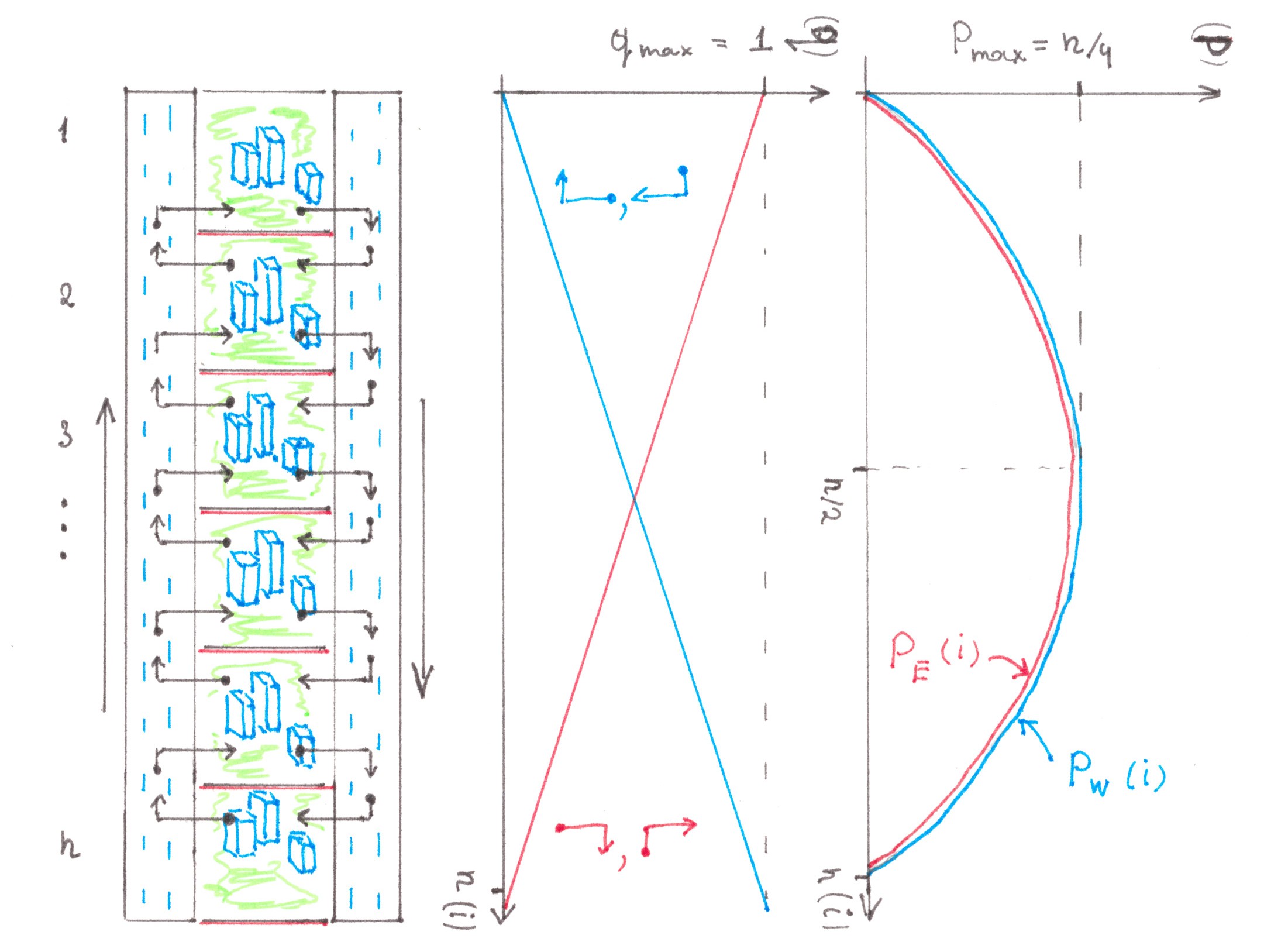
This time, we will consider an example of a city in which there are two one-way highways: Western highway with a traffic towards the north and Eastern highway with a traffic towards the south (Chart 25).
Chart 25
Let each quarter generate a flow with power 1. In this case, the power of one route heading from one quarter to another one amounts to 1/
n.
To begin with, we will define the power of side flows in the highways. Western highway is the only way to get to the quarter
i from the quarter (
n −
i) located southwards, and the only way to get from the quarter
i is to the quarter (
i − 1) located northwards. It means that the power of traffic exchange flows between Western highway and the quarter i are:
qW_out = (
n −
i)/
n — the power of the side flow leaving Western highway,
qW_in = (
i − 1)/
n — the power of the incoming side flow.
It is clear that the power of side flows in Eastern highway depends on i in a symmetrical way:
qE_out = (
i − 1)/
n — the power of the side flow leaving Eastern highway,
qE_in = (
n −
i)/
n — the power of the incoming side flow.
Of course, the sum of the flows leaving the
i-th quarter:
qE_in +
qW_in = (
n − 1)/
n,
coincides with the sum of the flows entering it:
qE_out +
qE_out = (
n − 1)/
n,
and both of these values do not depend on
i (each quarter has a flow with power 1/
n, this flow consists of trips which begin and finish within the given quarter).
To calculate the power of the main flows, we will draw an imaginary line across the Western highway on the same level with the
i-th quarter. In total, this line will cross:
(the number of quarters southwards) × (the number of quarters northwards) = (
n −
i)(
i − 1) of routes that together create a flow with the power:
PW(
i) = (
n −
i)(
i − 1)/
n.
The same formula:
(number of quarters southwards) × (number of quarters northwards)/
n,
should express the power of the traffic flow in the Eastern highway
PE, in other words:
PE(
i) =
PW(
i) =
P(
i).
Knowing the power of all the main and side flows, we can calculate the losses intensity rate that occur in the network in the area near the
i-th quarter:
I(
i) = (
α/2
ν)
⋅ P(
i)
⋅ [ (
qE_in +
qW_in)
⋅(1 + 1/
s) + (
qE_out +
qE_out)
⋅(1 − 1/
s) ] =
= (
α/2
ν)
⋅ P(
i)
⋅ [ (1 − 1/
n)
⋅ (1 + 1/
s) + (1 − 1/
n)
⋅ (1 − 1/
s) ] =
= (
α/2
ν)
⋅ 2
P(
i)
⋅ (1 − 1/
n) =
= 2(
α/2
ν)
⋅ (1 − 1/
n)
⋅ (
n −
i)(
i − 1)/
n =
= 2(
α/2
ν)
⋅ (1 − 1/
n)
⋅ (
n −
i)
⋅ (
i − 1)
⋅ (1/
n).
If we summarise the last expression across
i, we will get the losses intensity rate generated by the entire network as a whole.
I = ∑
i I(
i)
= ∑
i 2(
α/2
ν)
⋅ (1 − 1/
n)
⋅ (
n −
i)
⋅ (
i − 1)
⋅ (1/
n) =
= 2(
α/2
ν)
⋅ (1 − 1/
n)
⋅ n2 ⋅ ∑
i (1 −
i/
n)
⋅ (
i/
n − 1/
n)
⋅ (1/
n) ≈
≈ 2(
α/2
ν)
⋅ n2 ⋅ ∑
i (
i/
n)
⋅ (1 −
i/
n)
⋅ (1/
n).
The sum ∑
i (
i/
n)
⋅ (1 −
i/
n)
⋅ (1/
n) for any large
n can be replaced with good accuracy by the integral:
∫ t (1 −
t) d
t (
t∈[0; 1] ) = 1/2 − 1/3 = 1/6.
Based on this, we can obtain that the intensity of switching losses in a Linear city with
n quarters with power 1 amounts to:
I = (
α/2
ν)
n2/3.
Up to this point, we considered only examples in which quarters always generated flows with power 1. Let's consider if the formula for switching losses of a Linear city will change if for each quarter there is not one source of flow with power 1, but —
λ (the quarters will become
λ times larger).
Let us take a city with
m quarters. If quarters generated flows with power 1, then the switching losses would be (
α/2
ν)
m2/3.
An increase in trip production power by every quarter by a factor of
λ leads to an increase in both the main and side flows by a factor of
λ. As a result, the costs at each junction, and therefore inside the network as a whole, increase by a factor of
λ2 times, and the losses formula transforms into:
I = (
α/2
ν)
m2 ⋅ λ2/3.
To a large extent, it doesn’t matter how the switching losses depend on the number of quarters in the city, the main thing for us is how they depend on the flow power of all the trips generated inside it, or in other words, on the number
n of sources with power 1. In this case,
n is equal to
m⋅
λ, therefore:
I = (
α/2
ν)
m2⋅ λ2/3 =
= (
α/2
ν) (
m⋅λ)
2/3 =
= (
α/2
ν)
n2/3.
In other words, switching losses in a Linear city do not depend on how small the fragmentation of its territory into quarters is chosen.
Cellular city
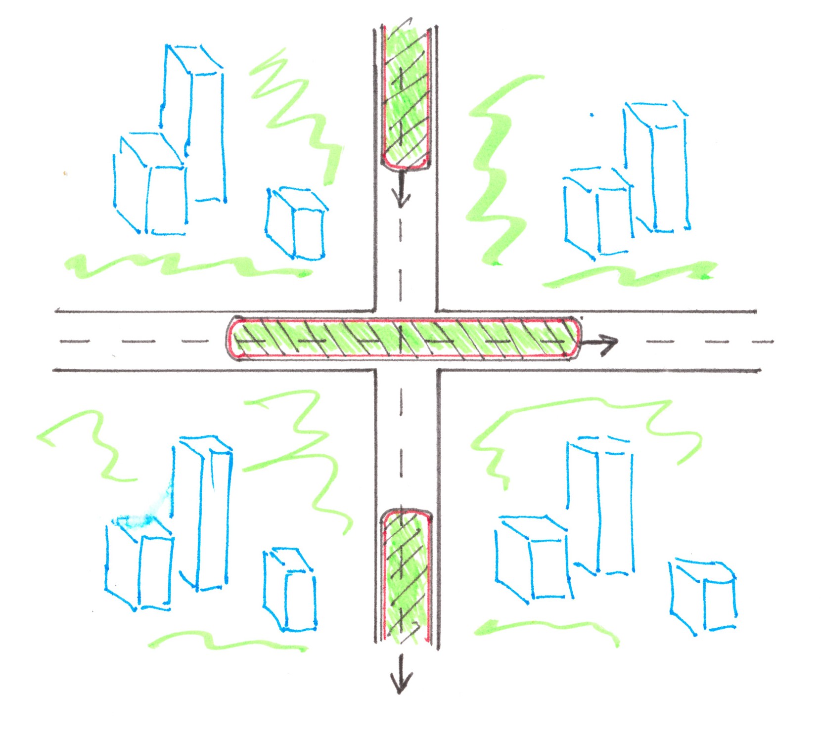
Imagine a Cellular city in which the highways of perpendicular streets are allocated at different heights/levels. This would be possible, for example, if all highways heading from north to south were raised on bridges, and highways stretching from west to east were built on the earth's surface. If, in addition, all highways have two-way traffic, then the road network in such a city will be referred to the standard Cellular topology (Chart 26).
The point here, of course, is not to bring the network described above seriously into practice: it would not look too aesthetically pleasing against the background of the city landscape and, moreover, due to the need for multi-level interchanges, it would eat up the better half of the street space. Nevertheless, this purely hypothetical network is a good way to get the necessary estimates, which later can be easily extended to road networks that are really interesting from the point of view of their applicability in real cities.
As usual, we will assume that the migration needs of residents are described by the 'random access' model, and we will start our consideration with the case when the power of all the flows generated by a given quarter is 1.
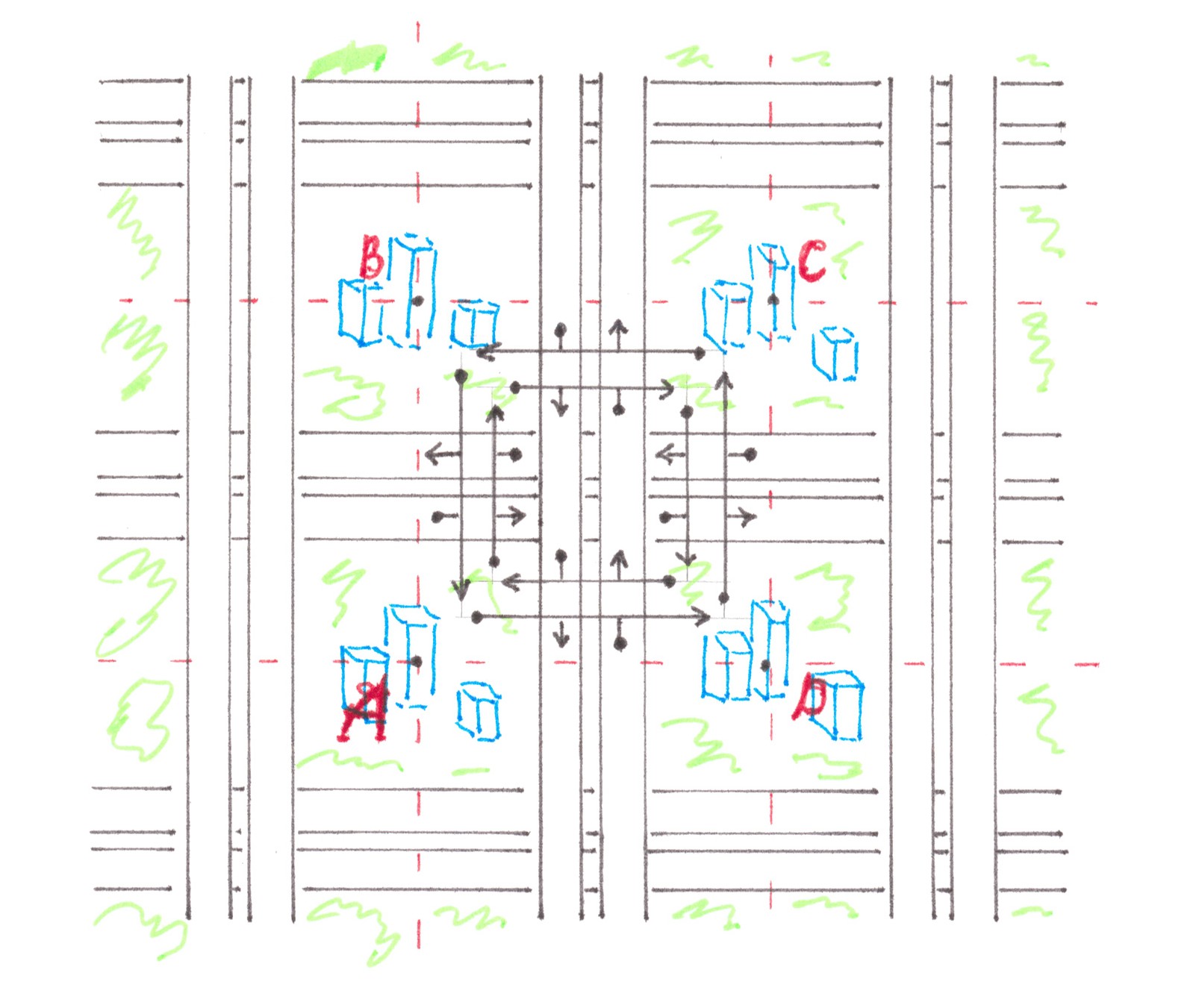
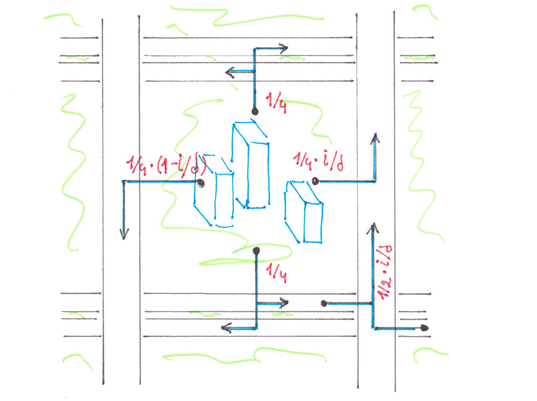
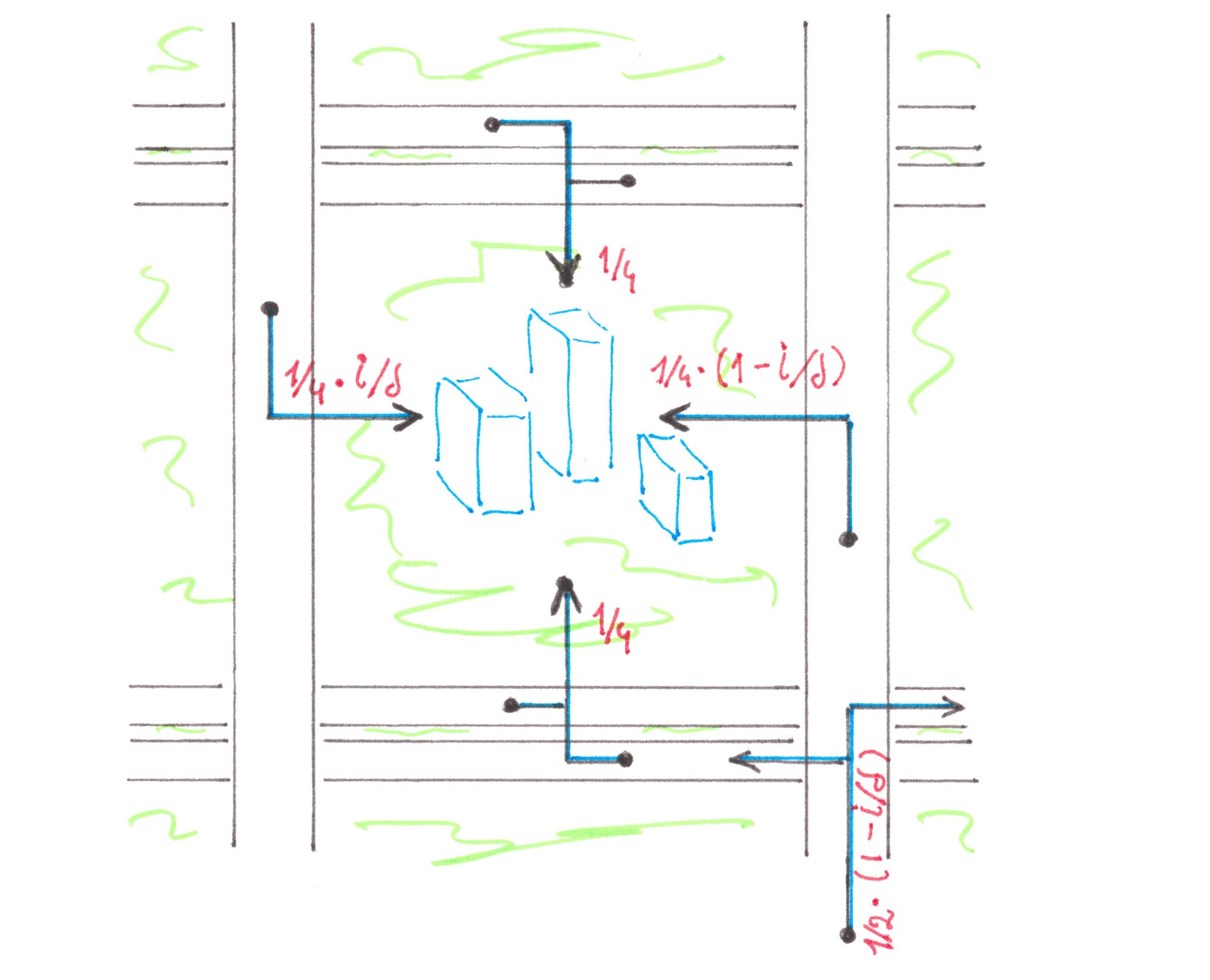
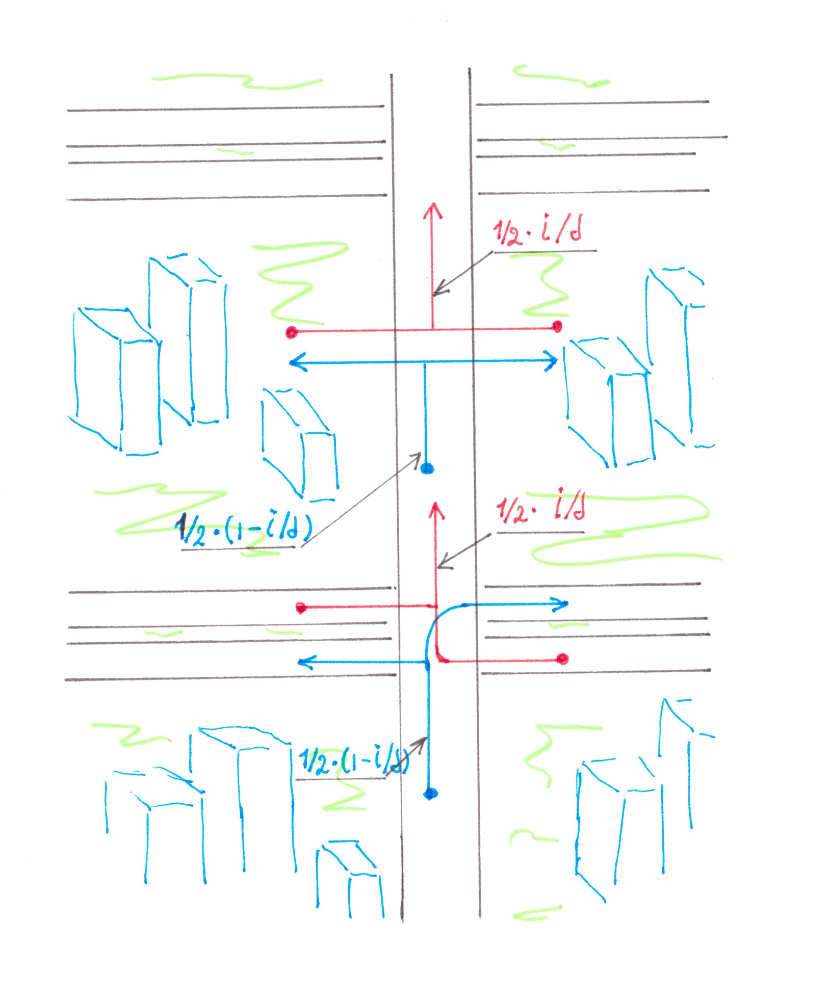
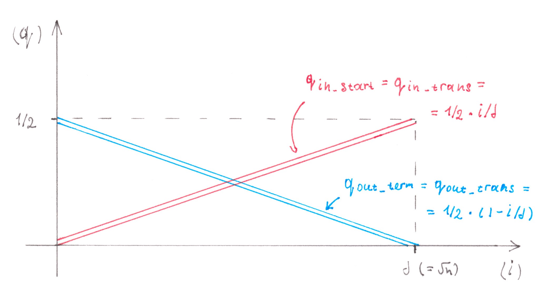
In the example of the standard Cellular city, it is convenient to step aside from the established tradition and consider as the address point not a separate quarter, but a territorial zone of a square shape within the intersection of highways and 1/4s of all quarters adjacent to it. Chart 27 shows the relative positioning of several such zones and shows a traffic pattern inside one of them. This chart clearly demonstrates that any driver, leaving the quarter, has the opportunity to enter in the highway, moving in the direction of any of the four sides of the world.
Chart 26
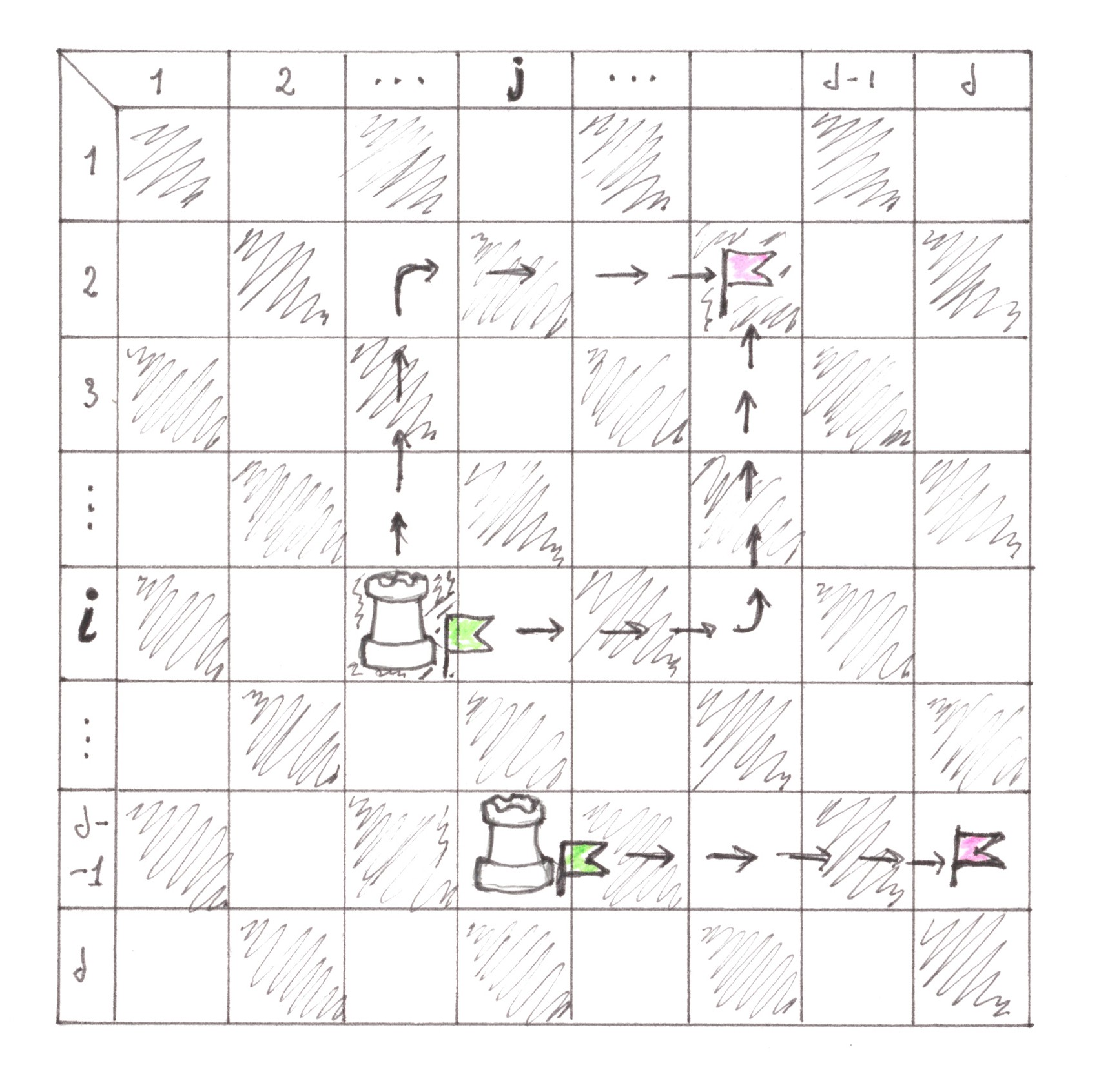
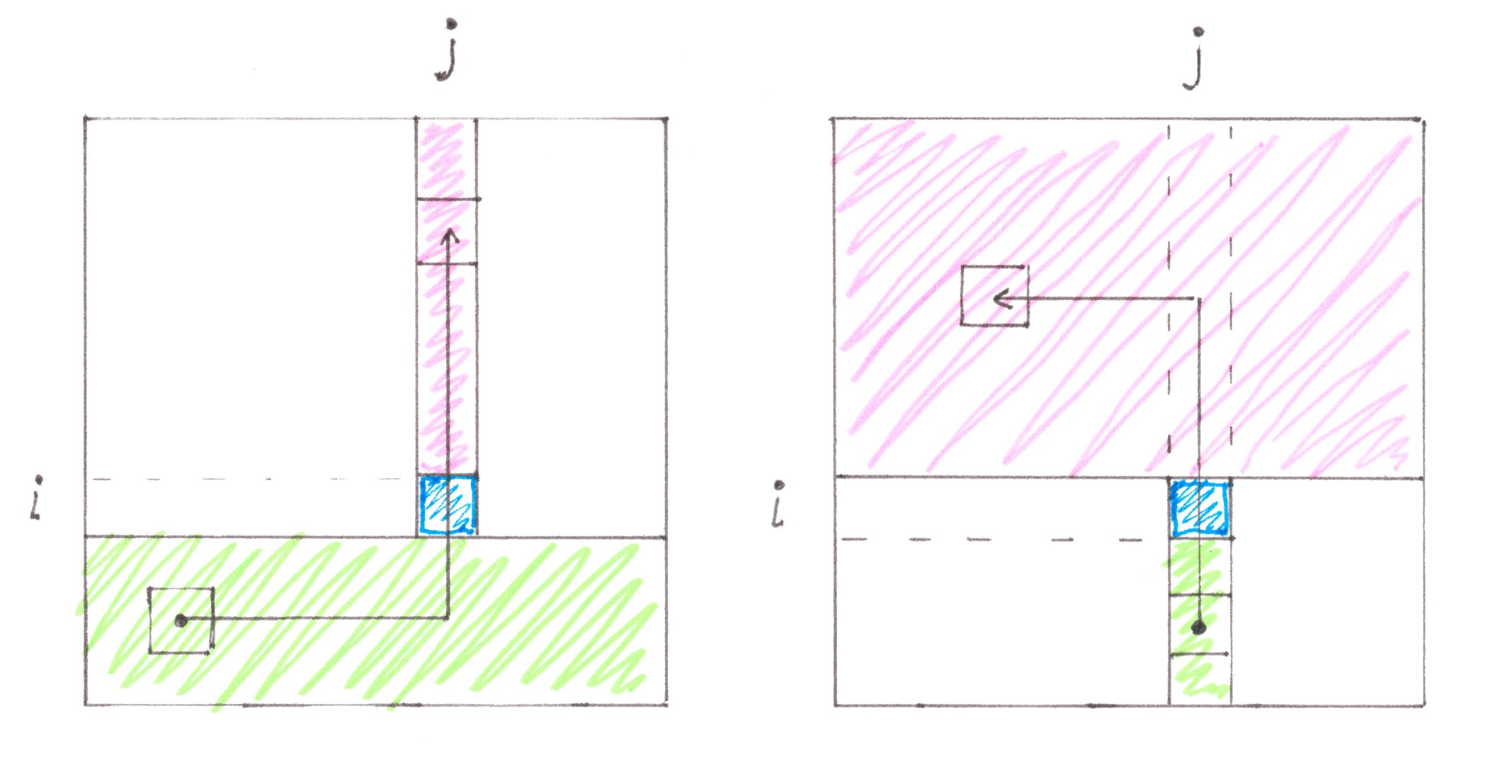
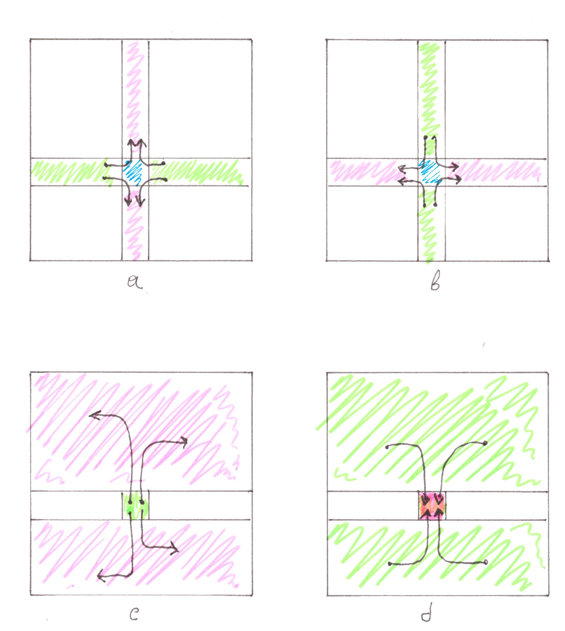
To calculate the value of switching costs generated by the city, we will calculate the power of all the main and side flows within each of its territorial zones. The shape and mutual positioning of the zones allow us to resort to a chess analogy to solve the problem in question, considering the zones as field cells, and the movement of cars between them — as movements of the rook (Chart 27). In a general case, the rook can be moved from one cell to another in two moves; if both cells are on the same horizontal or vertical line, then — in one move.
Chart 27
In order to avoid many inconvenient reservations, we assume that the move in which the rook does not move anywhere is also allowed according to our rules. The rook’s movement route, consisting of two moves, one of which is necessarily performed vertically, and the other -horizontally, will be called the simplest. It is reasonable to consider the move 'standstill' as vertical and horizontal at the same time. In this case, it turns out to be true that any two cells on the board are connected to each other by exactly two different simplest routes.
For drivers, the simplest route is the easiest way to get, with minimal interference, from one territorial zone to another, so it’s reasonable to assume that real trips will take place along elementary route lines. According to the 'random access' model, the flow with power 1 generated by the address point (territorial zone) should be equally distributed between all
n =
d2 address points of the city. Therefore, the power of the flow passing along one route line is 1/(2
n).
We can calculate the flow with what power passes through the cell (
i,
j ) in the direction from the south to the north. The simplest route crosses cell (
i,
j ) from the south to the north in only two situations. The first of them (Chart 28 on the left):
1a) the start cell of the route is located in one of the last (
d −
i) horizontal lines (rows);
2a) the finish point of the route is one of the first (
i − 1) cells of the
j-th vertical line (column);
3a) the route starts with a horizontal section, or lies entirely inside the
j-th column.
Chart 28
The conditions describing the second situation look symmetrical (Chart 28 on the right):
1a) the start point of the route is one of the last (
d −
i) cells of the
j-th vertical line;
2a) the finish cell of the route is located in one of the first (
i − 1) horizontal lines;
3a) the route starts with a vertical section, or lies entirely inside the
j-th column.
On the chessboard there is only 2× [
d⋅ (
i − 1) + 1⋅ (
i − 1) ] × (
d −
i) simplest routes suitable for the requirements, which together create a flow with the power:
PSN(
i,
j ) = (
d + 1)
⋅(
i − 1)
⋅(
d −
i) /
n ( =
PSN(
i ) ).
Fixing
j, we will obtain the function
(
PSN)
j (
i ) =
PSN(
i,
j = Const ),
describing the dependence of the power of the flow moving northwards along the
j-th vertical highway on the distance to the upper boundary of the city, measured in cells.
There are several more or less obvious observations regarding the functions (
PSN)
j (
i ), let's discuss them.
Let us start with a circumstance that would be difficult to overlook:
PSN(
i,
j ) practically independent on the second argument. As a result, the functions (
PSN)
j (
i ) =
PSN(
i ) have the same form for all values of
j, in other words, the specific position of the highway inside the Cellular city does not affect its load. Formally, the last statement is proved only for the highway heading to the north, but due to the symmetries of the city it automatically applies to the highway of other directions too.
Now let us look at the formula for
PSN(
i ) itself:
(
d + 1)
⋅(
i − 1)
⋅(
d −
i) /(2
n).
As we see, the whole dependence of
PSN от
ion i lies in the expression (
i − 1)
⋅(
d −
i). This expression can be interpreted as the product of the lengths of the right and left stretches into which the integer section of length d splits after the i-th element is excluded from it (Chart 29a).
Chart 29a
Chart 29b
It is clear that if you change “right” to “left” and “left” to “right” (Chart 29b), the result of the product will remain the same. Based on such a simple observation, we can draw two inferences that are, in essence, very useful for us:
- the function PSN( i ) is symmetric with respect to the midpoint of the street i = (d + 1)/2, in order words, the flow power at a distance Δ from the lower boundary of the city is exactly the same as at a distance from the lower boundary of the city is exactly the same as at a distance Δ from the upper boundary.
- On the whole, the city itself is symmetrical up and down, therefore, to get the function (PNS)j ( i ), which describes the power flow on the j-th highway, but in a southward direction, it’s enough to simply mirror the function graph (PSN)j ( i ) in the line i = (d + 1)/2. Since (PSN)j ( i ) = PSN( i ), and the graph PSN( i ) with respect to the line i = (d + 1)/2 is symmetric, then (PNS)j ( i ) = PSN( i ) = Pvert( i ),, in other words,
- direct and oncoming traffic flows have equal power at any point of the city. A closer graph of PSN( i )is shown in Chart 30 (it is believed that d >> 1, i >> 1, d − i >> 1).
Chart 30
The powers of the main flows along horizontal highways are easily found using rotational symmetries; formally, this process can be implemented through a simple replacement of
i by
j in
PSN(
i ) and a small correction of the lower index.
The next step to take is to find the power of the side flows. Trips that enter or leave traffic on a vertical highway inside the cell (
i,
j), can be conveniently divided into four categories:
- the flow qin_transit: start point is in any cell of the i-th horizontal, finish point is in any cell of the j-th vertical, except for the (i, j) itself (Chart 31a);
- the flow qout_transit: start point is in any cell of the the j-th vertical, except for the (i, j) itself, finish point is in any cell of the i-th horizontal (Chart 31b);
- the flow qin: start point is the (i, j) itself, finish one is any cell outside the i-th horizontal (Chart 31c);
- the flow qout: start point is in any cell outside the i-th horizontal, finish point is the (i, j) itself (Chart 31d);
Chart 32: a b c d
Having recounted the number of route lines belonging to each separate category, we can conclude that the powers of all four flows are the same and equal:
q0 =
d⋅ (
d − 1) /(2
n)
Having the values of the powers of the main and side flows in a vertical highway, it is not difficult to calculate the value of the respective switching costs. Inside a single cell (
i,
j ) the switching costs will be equal to:
Ivert(
i,
j ) = (
α/2
ν)
⋅ Pvert(
i )
⋅ [ (
qin +
qin_transit)
⋅(1 + 1/
s) + (
qout +
qout_transit)
⋅(1 − 1/
s) ] =
= 4 (
α/2
ν)
⋅ (
d + 1)(
i − 1)(
d −
i)
⋅ d(
d − 1) /2
n2 ≈
≈ 2 (
α/2
ν)
⋅ d5⋅ (
i/
d)(1 −
i/
d)
⋅ (1/
d)
4 =
= 2 (
α/2
ν)
⋅ d2⋅ (
i/
d)(1 −
i/
d)
⋅ (1/
d).
To find the costs incurred in all the vertical streets within the whole city, we need to sum
Ivert(
i,
j ) for both indices:
Ivert = ∑
ij Ivert(
i,
j ) =
= 2 (
α/2
ν)
⋅ d2⋅ ∑
ij (
i/
d)(1 −
i/
d)
⋅ (1/
d).
Since the value of the summands does not depend on
j in any way, summing over the second index is equivalent to multiplying by
d:
∑
ij (
i/
d)(1 −
i/
d)
⋅ (1/
d) =
d⋅ ∑
i (
i/
d)(1 −
i/
d)
⋅ (1/
d).
The last amount can be approximated by the integral that we already know:
∑
i (
i/
d)(1 −
i/
d)
⋅ (1/
d) ≈
∫ t (1 −
t) d
t (
t∈[0; 1] ) = 1/2 − 1/3 = 1/6.
Based on this, we can obtain:
Ivert = (
α/2
ν)
⋅ d3 /3 = (
α/2
ν)
⋅ n√
n /3.
We can answer the question what is the value of costs
Ihoriz, arising in the horizontal highways, using the symmetry of the city:
Ihoriz =
Ivert = (
α/2
ν)
⋅ n√
n /3.
Therefore, the switching losses intensity rate within the entire network of the Standard Cellular city is equal to:
I =
Ivert +
Ihoriz = 2/3
⋅ (
α/2
ν)
⋅ n√
n,
and per trip, on average, the switching costs will be
2/3
⋅ (
α/2
ν)
⋅√
n
The effect of cell size on the value of switching losses
Quarters generating flows with power 1 are a rather artificial limitation of the conditions of the problem. We can extend the results obtained above to the cases when the power of the flow generated by one cell is equal to
λ.
Let the city consist of
m such cells. If all cells were power 1, then the intensity of the total switching losses would be
I1 = 2/3
⋅ (
α/2
ν)
⋅ m√
m. An increase in the number of trips by a factor of
λ will multiply by
λ times the powers of all the main and side flows in the highways, which in turn will cause the increase by a factor of
λ2 in all the switching costs generated within the city. The new formula for the losses intensity rate will thus take the form:
I = 2/3
⋅ (
α/2
ν)
λ2⋅ m√
m
If we assume that the cell consists of
λ address points with power 1, then the total number of such points will be:
n =
λm. Let's express I as a function of
n and
λ:
I = 2/3
⋅ (
α/2
ν)
λ2⋅ m√
m =
= 2/3
⋅ (
α/2
ν)
⋅ √
λ⋅ (
λ√
λ)
⋅ (
m√
m) =
= 2/3
⋅ √
λ (
α/2
ν)
⋅ (
λm)√(
λm) =
= 2/3
⋅ √
λ (
α/2
ν)
⋅ n√
n.
The average cost per trip under the new conditions will be 2/3
⋅ √
λ (
α/2
ν)
⋅ √
n, being √
λ higher than their value in a city made up of quarters with power 1.
The last formula tells us that for the same population, population density and total area of all roads, the larger the size of the quarters chosen by its architect, the higher the switching costs. In the case when the city’s population is unevenly distributed over its territory, of course, we need to pay attention not to geometric dimensions, but first of all to the average number of people inside the quarter and their migration activity.
 (New York City Center photo: Vincent Laforet)
The remark made above is especially important when designing areas with skyscraper buildings. Due to the combination of high population density and its high mobility, it is crucial to design quarters in high-rise areas several times smaller in size than is usual for standard buildings. In civilizations, where skyscraper construction has a long history, the practice of isolating even separate large buildings as a quarter is widespread.
A cellular city with traffic light regulations
In each case, when the lines of two busy highways intersect on the map, the architect must make a choice: either lift one of these roads to the bridge, allowing the flow of the other to pass freely below, or realise the intersection in the form of an intersection, and resolve the flow conflict by traffic light regulation. The second option is often chosen in cities as it is attractively simple, does not imply the need to build large-scale engineering structures, and in addition it provides pedestrians with an easy way to cross the road.
 (деловые кварталы Лос-Анджелеса днем, фото: Борис Шеин)
The use of traffic lights in networks with cellular topology has its own characteristics. In Chapter 1, it was shown that with proper synchronisation of traffic lights, cars, while they are moving along the same street, do not even have to stop at intersections: a green light will always light in their direction. This kind of phenomenon is usually called the green wave traffic management. To create it, traffic flows need to be divided into two alternating: filled with cars and free of them. Next, such a mode of traffic lights operation is selected that in the period of time when the next “portion” passes the intersection along one of the streets, the previous portion of cars moving along the perpendicular street has already passed it, and the next one has not yet arrived (Chart 33).
Chart 33
Green wave traffic management carries its own costs and imposes certain restrictions on the layout of city streets.
Looking again at Chart 33, it is easy to see that at any given time exactly half of the area of all roads is not actually used. To compensate this downtime, in the actively used half, the local power of car flows and the number of lanes necessary for them should be twice as large as in a city with overpasses.
The second most important circumstance associated with the use of green waves is the strict regulation of the permissible size of quarters: their length (for two-way streets) should be a multiple of the length of the filled green wave (a section of the flow within which unhindered movement is possible), amounting to about 500 metres. As noted in the previous paragraph, areas with a high population density require an increased frequency of location of roads, so the restriction on the distance between highways (the permissible size of quarters) can potentially cause traffic difficulties.
It is interesting to note that in the green wave traffic management, the switching rules inside the network slightly change. For example, the addition of one more car to the main traffic flow can be performed in the intervals between the filled zones, without thereby causing any serious switching costs (point 1 in Chart 34a).
Chart 34
Of course, this car itself will have to lose some time waiting for the nearest empty zone before getting into the highway, and after that stand at the traffic light until the next filled zone hits it (point 2, Chart 34a), however the value of these losses does not depend either on the size of the city or on the busyness of traffic in the street, therefore, they can be neglected on a large scale.
The situation is completely different if a car tries to leave the highway traffic (Chart 34b). Here, apparently, there are no longer any tricky ways how to make the switching losses created by the driver less. Moreover, due to the doubling of the local power of the flow inside the filled zones, leaving of a randomly selected car from it causes time costs twice as much as in a city with overpasses. In total, the cheaper “entry” and more expensive “exit” offset each other, making the Traffic Light Cellular city in this respect almost no better, but no worse than Standard one.
Flyover Cellular city with one-way traffic
In addition to the use of traffic lights, there is at least one more opportunity to avoid the monstrous interchanges of the Standard city. It implies dividing spatially two-way highways (Chart 35).
Chart 35
As a result of such changes, the number of streets will double, they will all become one-way streets, but most importantly, the interchanges will be greatly simplified (Chart 36).
Chart 36
Since the number of highways heading to each of the sides of the world and the number of journeys passing along them remained the same, the powers of all flows together with the switching costs in the One-way Cellular city and the Standard city with 2 times larger (linearly) quarters, should coincide. If we compare the Standard and the One-way cities with the same quarter sizes, then the switching losses in the second one will be twice as high.
Advanced Road Networks
«Linear» street
How could switching losses be reduced in a Cellular network? The answer to this question can be find by selecting a correct analogy, with the help of a little savvy.
Let us consider a somewhat unusual modification of the Cellular network, which implies that all highways stretching from west to east are two-way, while the perpendicular to them highways are only one-way: either north or south, and these directions alternate from street to street.
As always, we will assume that the city follows the random access model, and each quarter of it generates a flow with power 1.
In this case, it seems quite plausible that the flow originated inside the quarter (
i,
j ) is distributed between the nearest streets as follows: 1/4 of it will go to the horizontal road northwards, 1/4 — to the horizontal road southwards, 1/4⋅
i/
d — to the vertical highway to the north and 1/4 ⋅ (1 —
i/
d) — to the second vertical highway to the south (Chart 37).
Chart 37
Indeed, according to the previously discussed route algorithms, according to statistics, half of the journeys will start from a horizontal section, and for drivers who would prefer this half, it should to a large extent not matter whether their path lies northwards or southwards of the quarter (
i,
j ). The remaining half of the journeys will start from a vertical section of traffic and will be divided between highways heading to the south and north as a ratio of the number of quarters lying southwards from the quarter (
i,
j ) to the number of quarters lying northwards from it.
As to the flow of trips heading inward the quarter (
i,
j ), the rule of its division with respect to the highways surrounding the quarter will be symmetrical (Chart 38).
Chart 38
Among the four intersections adjacent to the quarter (
i,
j ), we can consider separately the lateral flows at the intersection of the lower horizontal highway and the vertical street with traffic to the north (Chart 38). The flow of cars entering into the intersection and heading from the horizontal street to the vertical one is:
1/2⋅ (number of quarters on the horizontal)×( number of quarters on the vertical not lower than (
i,
j ))
⋅ 1/
d2 =
= 1/2
⋅ d⋅ i/
d2 =
= 1/2
⋅ i/
d.
The power of lateral flow in the opposite direction is:
1/2⋅ (the number of quarters on the vertical is strictly lower than (
i,
j ))×(the number of quarters on the vertical)
⋅ 1/
d2 =
= 1/2
⋅ (
d −
i)
⋅ d/
d2 =
= 1/2
⋅ (1 −
i/
d).
Let’s now turn our attention from the Cellular city as a whole to any one of its vertical streets, let's call it My_street. By virtue of symmetries, we will not limit our reasoning in any way, if we assume that the movement along My_street is directed from south to north (Chart 39).
Chart 39
Chart 40 depicts the power of the main and side flows on the highway along My_street, which, as the reader may notice, are incredibly similar to similar graphs for the one-way highway of a Linear city (Chart 26).
Chart 40
In these examples, the flow diagrams coincide completely if inside My_street the lateral flows relating to each pair of opposing quarters and the horizontal highway below them are formally assigned to one imaginary territorial cell. As can be seen from the earlier tables, the road network of a Linear city generates some of the largest switching losses among the networks we have already studied. From this point of view, the traffic pattern within the boundaries of a single street of a Cellular city looks extremely inefficient and is an element that should be improved in the first place.
Advanced Linear City Network
So, we are facing the task of improving a Linear network so that it does not turn into a «square» one. The circumstance that represents the greatest inefficiency in the operation of the Linear Network is the merging of all routes into only two very large traffic flows. In this situation, a reasonable step would be to divide the flows along both of its street highways into
Q equal parts. Since the time costs caused by each car joining or leaving traffic are proportional to the traffic intensity on it, as a result of dividing the street lines into
Q isolated parts (Chart 41a), the switching losses inside a Linear city should have decreased
Q times.
Chart 41
Even after the construction of ten roads nearby we can't hope that the drivers themselves will be equally distributed between them — unfortunately, it does not seem to have a chance of success. A much more thoughtful decision would be to design the network so that each road does not lead to all quarters, but only to a small “segment” of the city, where it would be difficult to get to without using the given road (Chart 41b).
You can see a similar idea in the scheme of movement of elevators inside multi-storey buildings where each elevator allows you to enter and exit it not on all floors, but only within a certain range of heights. Accepting this concept, let us take a closer look at the road
rk, which gives access to the segment
Δk = (
xk,
xk +1 ] for trips that started (not strictly) southwards from xk (it is believed that the numbering of the quarters is performed from the bottom up).
From each quarter which number is fewer (not strictly) than
xk, a
qin stream with a power of
Δk|/
n ( по 1/
n to each quarter inside
Δk ) enters the road
rk, at the same time it is assumed that there is no possibility to turn from
rk towards any of the mentioned quarters either due to established traffic rules, or due to a special design of the road network.
The cars accumulated on the segment [1,
xk] will eventually be evenly distributed between the quarters inside
Δk, therefore, if there were no trips whose start and finish points lie inside
Δk, then the side flows
qout in the direction of each of the quarters in this section would have the power
xk/
n (Chart 42).
Chart 42
In fact, the contribution of “internal” trips to the power of side flows does exist, however, the value of this contribution never exceeds |
Δk|/
n, therefore, in the case when
xk >> |
Δk|, it can be simply neglected. The power
pk of the main stream along
rk with simplifications made will be represented by a graph of two straight sections with a maximum
Pk equal to
xk⋅ |
Δk|/
n. The approximate value of switching losses in the road
rk can be found by the formula:
Ik = (
α/2
ν)
⋅ ∑x[
qin(
x)
⋅ pk(
x)
⋅ (1 + 1/
s) ] + (
α/2
ν)
⋅ ∑x[
qout(
x)
⋅ pk(
x)
⋅ (1 − 1/
s) ] =
= (
α/2
ν)
⋅ (1 + 1/
s)
∑x[ |
Δk|/
n⋅ pk(
x) ] + (
α/2
ν)
⋅ (1 − 1/
s)
∑x[
xk/
n⋅ pk(
x) ] =
= (
α/2
ν)
⋅ (1 + 1/
s)
⋅ (
xk⋅ |
Δk|/
n)
⋅ (
∑xpk(
x) )/
xk + (
α/2
ν)
⋅ (1 − 1/
s)
⋅ (
xk⋅ |
Δk|/
n)
⋅ (
∑xpk(
x) )/|
Δk|,
where the first sum is taken over a segment
x ∈ [1,
xk], and the second over
x ∈
Δk. The expressions:
(
∑xpk(
x) )/
xk,
x∈ [1,
xk] and
(
∑xpk(
x) )/|
Δk|,
x∈
Δk
are nothing other than the average power of the flow along
rk inside the indicated intervals. Since the power graph within these intervals has the form of a straight line, the average power in both cases is
Pk/2. Replacing
xk⋅ |
Δk|/
n by
Pk,
we finally present the formula for losses intensity rate in its simplest form:
Ik = 2 (
α/2
ν)
⋅ Pk⋅ Pk/2 = (
α/2
ν)
⋅ Pk2
Let us now try to calculate the sequence
xk of numbers of those quarters by which a linear city should be divided into segments. As a criterion for the selection of segments, we can take the requirement that the maximum power of the traffic flows
Pk in the roads approaching them should have the same value, independent of
k, in other words:
xk⋅ |
Δk| = Const.
Remembering that |
Δk| =
xk + 1 −
xk, we can infer the difference equation:
xk + 1 −
xk = Const/
xk.
Assuming
x and
k are continuous variables, and replacing
xk + 1 −
xk =
x(
k + 1) −
x(
k)
by d
x/d
k⋅ 1,
we can approximate the difference equation by the differential one:
d
x/d
k = Const/
x <=>
xd
x = Const
⋅ d
k.
from which we can infer a solution for
xk in the general form:
xk = С
1 √(
k + С
2).
It remains for us to determine the value of the constants С
1 and С
2 based on their boundary conditions, however, there is an important subtlety in this matter. Unlike the situation in other segments, all the cars arriving from the western highway to the quarters of the segment with number 1, began their trips inside the same segment. As a result, the graph of the flow power in the first highway to the north will have the form of a regular inverted parabola.
At the same time, the a priori conditions from which the formula for
xk was obtained essentially assumed that the flow power graphs on all highways should be close to a triangular view, and the trips themselves should begin mainly outside the segment where they are directed to. These requirements can be fulfilled with reasonable accuracy if we formally divide the first segment into two equal parts, without increasing the number of roads. Most of the trips that take place along the first highway begin in its southern half, and end in the northern half. Considering only them, we thereby do not make a big mistake in calculating the switching losses, but now the power diagram of the main flow will have just a triangular shape (Chart 43).
Chart 43
It is the middle of the first segment that should be considered the point
x1 in the formula for
xk. This allows us to get the first boundary condition:
x2 = 2
x1 or
√( 2 + С
2) = 2
⋅ √( 1 + С
2) =>
С
2 = − 2/3.
The second boundary condition can be obtained from the requirement that the roads and segments of everything are exactly
Q, which means
xQ + 1 should be subsequent to the quarter with the largest number in the city:
С
1 √(
Q + 1 − 2/3) =
n + 1, whence
С
1 ≈ (
n + 1)/√
Q.
Therefore:
xk ≈ (
n + 1)
⋅ √(
k − 2/3)/√
Q,
|
Δk| ≈ d
x/d
k = (
n + 1)/ 2√(
k − 2/3)
⋅√
Q
Pk =
xk⋅ |
Δk|/
n =
= (
n + 1)
2/ 2
n⋅ Q ≈
n/ 2
Q
Ik = (
α/2
ν)
⋅ Pk2 =
= (
α/2
ν)
⋅ (
n/ 2
Q)
2.
Since all 2
Q highways generate losses of the same intensity, the value of switching costs within the entire network will be:
I = 2
Q⋅ (
α/2
ν)
⋅(
n/ 2
Q)
2 = (
α/2
ν)
⋅ n2/ 2
Q.
As you can see, the desired result has been achieved: after dividing the main highways into
Q parts, the losses indeed decreased by a factor of
Q (except for the increased from 1/3 to 1/2 constant coefficient, compared to the formula for the usual Linear city). Well, we are halfway there, it remains only to apply this result to improve the city with Cellular architecture.
'Skyscraper Elevator' in a Cellular city
For simplicity, we will consider an example of a city in which all the streets are one-way. Using the analogy between a Linear city and the individual streets of a Cellular city, we can divide the highway along the latter into
Q parts. By default, it is believed that leaving the quarter, the driver can choose any highway passing near it. At the same time, among all the highways laid along one street, there is a turn towards a specific quarter from exactly one of them. In the process of establishing rules, their uniformity and simplicity are extremely important. Let's take a look at Chart 44:
Chart 44
all the streets have the same view and the same rules as to which of the roads opens access onto which quarter. Chart 45 shows a diagram of permitted turns between highways. Looking at this picture, it is hard not to get confused. The same is often said about the underground scheme in some large city. However, in both cases, everything becomes clear and simple if you know the logic of the idea. The logical rule of permitted turns sounds quite simple: if driving along a highway, you cross roads perpendicular to your movement and you can turn into a quarter located directly behind them, you can turn into any of these roads.
Chart 45
The 'Skyscraper elevator' topology is compatible with both traffic light intersections and overpasses. It is difficult, but possible to generalise it to networks not necessarily of a cellular or linear structure. The latter is really important for historical cities, where it is unlikely that it would be a right decision to demolish half of the historical monuments in order to design many small straight streets, but in which there are already quite large streets that can accommodate several two- or three-lane highways.
About the transport problems and the work of a mathematician
It is pleasant to complete the 6 months laborious work. The work I wrote, of course, does not solve all the problems and difficulties of road design — this issue requires a large number of very versatile and multi-skilled people. Nevertheless, its results provide an opportunity to see important errors in already built cities and provide methods of how to avoid such errors in the future. This article was not intended as a reference book covering all possible cases that an engineer can face in practice — I considered my main aim is to give a new point of view, to develop a new way to reason and talk about the problem, to provide the reader with the necessary minimum of simple model examples which could be expanded by the reader further.
It becomes sad when you realise how much time was lost by city residents in traffic jams just because at the right time there was no mathematician who could spend the evening on a completely solvable problem. How many such problems still surround our life or hide in your profession? Is a person sitting near you at work whose tools are a pencil and a sheet of paper?
I hope everything will change for the better.
I would like to express my sincere gratitude to Janine Lacroix (pseudonym) for her work on translating this text from its original Russian to English.
Thank you for your attention and good luck!
Sergei Kovalenko
2019
magnolia@bk.ru

(Фото: Vincent Laforet)


